Return to computing page for the second course APMA0340
Return to computing page for the fourth course APMA0360
Return to Mathematica tutorial for the first course APMA0330
Return to Mathematica tutorial for the second course APMA0340
Return to Mathematica tutorial for the fourth course APMA0360
Return to the main page for the course APMA0330
Return to the main page for the course APMA0340
Return to the main page for the course APMA0360
Return to Part I of the course APMA0330
Glossary
Parametric Plots
A parametric equation defines a group of quantities as functions of one or more independent variables called parameters. Parametric equations are commonly used to express the coordinates of the points that make up a geometric object such as a curve or surface, in which case the equations are collectively called a parametric representation or parameterization (British English: "parametrisation") of the object. Mathematica has a dedicated command for these purposes: ParametricPlot.
You can display many functions using implicit methods. Explicitly defined functions can be plotted using the regular Plot command.
|
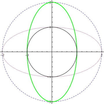
Labeled[ParametricPlot[{{2 Cos[t], 2 Sin[t]}, {2 Cos[t],
Sin[t]}, {Cos[t], 2 Sin[t]}, {Cos[t], Sin[t]}}, {t, 0, 2 Pi},
PlotStyle -> {Dashed, Dashing[Tiny], Directive[Thick, Green],
Black}], "Circles and elipses"]
You can use the option Plotlegent to identify equations in use.
ParametricPlot[{{2 Cos[t], 2 Sin[t]}, {2 Cos[t], Sin[t]}, {Cos[t],
2 Sin[t]}, {Cos[t], Sin[t]}}, {t, 0, 2 Pi},
PlotStyle -> {Dashed, Dashing[Tiny], Directive[Thick, Green], Black},
PlotLegends -> "Expressions"]
|
You can enjoy using a newer Mathematica package: NotebookEmbedder from Wolfram Cloud notebooks on websites. An HTML Mathematica package, NotebookEmbedder, permits you to place notebooks stored in the cloud in your website. Wolfram offers a wide range of options.
The input element
Click the "Submit" button and the form-data will be sent to Wolfram Cloud at this specific URL to generate a plot and return the result as a PNG image".
Alternate view in animation form
|
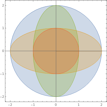
Or you can make a similar plot with overlapping regions:
ParametricPlot[{{2 r Cos[t], 2 r Sin[t]}, {2 r Cos[t],
r Sin[t]}, {r Cos[t], 2 r Sin[t]}, {r Cos[t], r Sin[t]}}, {t, 0,
2 Pi}, {r, 0, 1}, Mesh -> False]
|
|
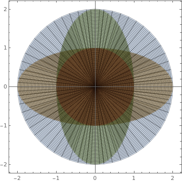
Another option:
ParametricPlot[{{2 r Cos[t], 2 r Sin[t]}, {2 r Cos[t],
r Sin[t]}, {r Cos[t], 2 r Sin[t]}, {r Cos[t], r Sin[t]}}, {t, 0,
2 Pi}, {r, 0, 1}, Mesh -> All]
|
|
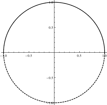
ParametricPlot[{Cos[t], Sin[t]}, {t, 0, 2 Pi},
PlotStyle -> Directive[Thick, Black], Mesh -> {Range[0, 2 Pi, Pi]},
MeshShading -> {Dashed, {}}]
|
We can place our plots in a row:
pp2 = Labeled[ ParametricPlot[{{2 r Cos[t], 2 r Sin[t]}, {2 r Cos[t], r Sin[t]}, {r Cos[t], 2 r Sin[t]}, {r Cos[t], r Sin[t]}}, {t, 0, 2 Pi}, {r, 0, 1}, Mesh -> All], "Showing mesh elements used in sampling"];
pp3 = Labeled[ ParametricPlot[{Cos[t], Sin[t]}, {t, 0, 2 Pi}, PlotStyle -> Directive[Thick, Black], Mesh -> {Range[0, 2 Pi, Pi]}, MeshShading -> {Dashed, {}}], "Segments of curves with different styles"];
GraphicsRow[{pp1, pp2, pp3}, ImageSize -> 700]
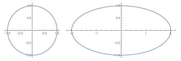
Sin waves, parabolas, circles, arcs and ellipses are just special cases of the more general concept of "curve." Here are a circle and an ellipse. Note that the independent variable, t, must be the same within each equation. Both x and y must be parameterized by t, one may not, for instance, parameterize x by t and y by s.
pp4 = ParametricPlot[{x, y}, {t, 0, 2 Pi}];
pp5 = ParametricPlot[{2*x, y}, {t, 0, 2 Pi}];
GraphicsRow[{pp4, pp5}]
Also, we can plot
|
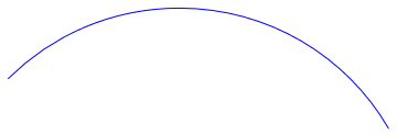
Actually, there is a special command in Mathematica that can be used to plot circles and ellipses:
Circle[{x,y},r] gives a circle of radius r centered at {x,y}. Circle[{x,y}] represents a circle of radius 1. Circle[{x,y},{r_x , r_y}] gives an axis-aligned ellipse with semi-axes length r_x and r_y. Circle[{x,y},..., {theta_1 , theta_2}] gives a a circular or ellipse arc from angle theta_1 to theta_2
Graphics[{Blue, Circle[{0, 1}, 2, {Pi/6, 3*Pi/4}]}]
|
|
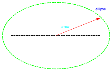
R = Graphics[{Green, Thick, Dashed,
Circle[{1, 2}, {1.2, 0.75}], {Blue,
Inset["ellipse", {2, 2.6}]}, {Black, Line[{{0, 2}, {2, 2}}]}}]
a = Graphics[{Red, Arrow[{{1, 2}, {2, 2.4}}], {Cyan, Text[arrow, {1.2, 2.2}]}}] Show[R, a] |
There are special commands in Mathematica that can be used to plot circles and ellipses:
Circle[{x, y}, r] gives a circle of radius r centered at {x, y} .Circle[{x, y}] represents a circle of radius 1.
Circle[{x, y}, {r_x, r_y}] gives an axis - aligned ellipse with semi - axes length r_x and r_y .
Circle[{x, y}, ..., {theta_ 1, theta_ 2}] gives a a circular or ellipse arc from angle theta_ 1 to theta_ 2
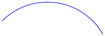
a = Graphics[{Red, Arrow[{{1, 2}, {2, 2.4}}], {Cyan, Text["arrow", {1.2, 2.2}]}}];
Labeled[Show[pp6, a], "Ellipse with text"]
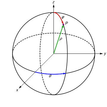
To visualize spherical coordinates, use the following codes:
|
circle[x_] = {Cos[x], Sin[x]};
ellipsePhi[x_, a_: - Pi/2] = {Cos[x - a]/3, Sin[x + a]};
ellipseTheta[x_, a_: 0] = {Cos[x + a], Sin[-x - a]/2};
ParametricPlot[circle[x], {x, 0, 2 Pi}, PlotStyle -> Black,
Epilog ->
First /@ {(*Ellipses*)
ParametricPlot[{ellipsePhi[x], ellipsePhi[-x], ellipseTheta[-x],
ellipseTheta[x]}, {x, 0, Pi},
PlotStyle -> {{Black, Dashed}, Black}],(*Co-ordinate axes*)
Graphics[
Table[GeometricTransformation[{Arrowheads[0.03],
Arrow[{{0, 0}, {1.2, 0}}]},
ReflectionMatrix[circle[x]]], {x, {Pi/2, -Pi/4, Pi/8}}]],
(*mark point,rho,phi& theta directions*)
ParametricPlot[{ellipsePhi[x, Pi/2],
ellipseTheta[-x, 13 Pi/20]}, {x, 0, Pi/4},
PlotStyle -> {{Red, Thick}, {Blue, Thick}}] /.
Line[x__] :> Sequence[Arrowheads[0.03], Arrow[x]],
Graphics[{{Directive[Darker@Green, Thick], Arrowheads[0.03],
Arrow[{{0, 0}, ellipsePhi[-3 Pi/4]}]}, {Directive[Purple],
Disk[ellipsePhi[-3 Pi/4], 0.02]}}],
(*text*)
Graphics[{Text[Style["x", Italic, Larger], 1.25 circle[5 Pi/4]],
Text[Style["y", Italic, Larger], 1.25 circle[0]],
Text[Style["z", Italic, Larger], 1.25 circle[Pi/2]],
Text[Style["\[Rho]", Italic, Larger], 0.4 circle[4 Pi/11]],
Text[Style["\[CurlyPhi]", Italic, Larger],
1.1 ellipsePhi[Pi + Pi/5]],
Text[Style["\[Theta]", Italic, Larger],
1.1 ellipseTheta[13 Pi/20 - Pi/8]],
Text[Style["P", Italic, Larger], 1.2 ellipsePhi[-3 Pi/4 + Pi/24]]}]
}, Axes -> False, PlotRange -> 1.3 {{-1, 1}, {-1, 1}}
]
|
This alternative solution has the advantage of being created using 3D directives. As such, it was easy to wrap inside a Manipulate and you can drag it with your mouse to change the viewpoint:
Another way to think about parametric plots is that it allows one to "sneak" a fourth variable into a plot of a three dimensional figure. To visualize this using spherical coordinates, below you see three axes, x, y and z, each parameterized by a fourth variable, t:
Alternative plot:
ellipsePhi[t_, a_ : -Pi/2] = {Cos[t - a]/3, Sin[t + a]};
ellipseTheta[t_, a_ : 0] = {Cos[t + a], Sin[-t - a]/2};
pp7 = ParametricPlot[{circle[t], ellipsePhi[t, a], ellipseTheta[t, a]}, {t, 0, 2 Pi}, PlotStyle -> Black, Epilog -> First /@ {(*Ellipses*) ParametricPlot[{ellipsePhi[x], ellipsePhi[-x], ellipseTheta[-x], ellipseTheta[x]}, {x, 0, Pi}, PlotStyle -> {{Black, Dashed}, Black}],(*Co-ordinate axes*) Graphics[ Table[GeometricTransformation[{Arrowheads[0.03], Arrow[{{0, 0}, {1.2, 0}}]}, ReflectionMatrix[circle[x]]], {x, {Pi/2, -Pi/4, Pi/8}}]],(*mark point,rho,phi& theta directions*) ParametricPlot[{ellipsePhi[x, Pi/2], ellipseTheta[-x, 13 Pi/20]}, {x, 0, Pi/4}, PlotStyle -> {{Red, Thick}, {Blue, Thick}}] /. Line[x__] :> Sequence[Arrowheads[0.03], Arrow[x]], Graphics[{{Directive[Darker@Green, Thick], Arrowheads[0.03], Arrow[{{0, 0}, ellipsePhi[-3 Pi/4]}]}, {Directive[Purple], Disk[ellipsePhi[-3 Pi/4], 0.02]}}],(*text*) Graphics[{Text[Style["x", Italic, Larger], 1.25 circle[5 Pi/4]], Text[Style["y", Italic, Larger], 1.25 circle[0]], Text[Style["z", Italic, Larger], 1.25 circle[Pi/2]], Text[Style["\[Rho]", Italic, Larger], 0.4 circle[4 Pi/11]], Text[Style["\[CurlyPhi]", Italic, Larger], 1.1 ellipsePhi[Pi + Pi/5]], Text[Style["\[Theta]", Italic, Larger], 1.1 ellipseTheta[13 Pi/20 - Pi/8]], Text[Style["P", Italic, Larger], 1.2 ellipsePhi[-3 Pi/4 + Pi/24]]}]}, Axes -> False, PlotRange -> 1.3 {{-1, 1}, {-1, 1}}]
Return to Mathematica page
Return to the main page (APMA0330)
Return to the Part 1 (Plotting)
Return to the Part 2 (First Order ODEs)
Return to the Part 3 (Numerical Methods)
Return to the Part 4 (Second and Higher Order ODEs)
Return to the Part 5 (Series and Recurrences)
Return to the Part 6 (Laplace Transform)
Return to the Part 7 (Boundary Value Problems)