This section presents a technique to find a particular solution to the driven linear constant coefficient differential equation when its nonhomogebeous term has a special form: polynomial times exponential function times a trigonometric function. The technique, called the
method of undetermined coefficients, reduces the problem down to an algebra problem.
Return to computing page for the first course APMA0330
Return to computing page for the second course APMA0340
Return to Mathematica tutorial for the first course APMA0330
Return to Mathematica tutorial for the second course APMA0340
Return to the main page for the course APMA0330
Return to the main page for the course APMA0340
Return to Part IV of the course APMA0330
Let \( \texttt{D} = {\text d}/{\text d}x \) be the derivative operator and its powers are defined recursively:
\( \texttt{D}^{m+1} = \texttt{D} \left( \texttt{D}^{m} \right) , \quad m=0,1,2,\ldots . \) As usual, its zero power is identified with the identity operator \( \texttt{D}^{0} = \texttt{I} , \) where I is the identity operator:
I(f) = f for any function f.
We consider linear constant coefficient differential operators that are
generated by a polynomial of degree n:
It is always assumed that the coefficients of the above operator are
constants. Moreover, we always suppose
that the leading coefficient 𝑎n ≠ 0. Therefore, it could be factored out or set to be 1.
The Idea why the Method of Undetermined Coefficients works
We know from the previous section that the general solution of the nonhomogeneous differential equation
\[
L \left[ \texttt{D} \right] y = f(x) \qquad \mbox{or} \qquad a_n y^{(n)} + a_{n-1} y^{(n-1)} + \cdots + a_1 y' + a_0 y = f(x)
\]
is the sum of yh(x), the general solution of the homogeneous equation \( L \left[ \texttt{D} \right] y_h = 0, \) and yp(x), a particular solution of the driven equation \( L \left[ \texttt{D} \right] y_p = f(x). \) We also know how to find the general solution of the homogeneous equation \( M \left[ \texttt{D} \right] y_h = 0 \)
for any constant coefficient differential operator M because it is
actually reduced for solving the polynomial equation
\( M \left( \lambda \right) = 0 . \)
If the input function f(x) is known to be annihilated by some constant coefficient differential operator M:
then we can reduce the given problem to the known problem for solving homogeneous differential equation (ML) y = 0. To achieve this, we just multiply the given nonhomogeneous equation
\( L \left[ \texttt{D} \right] y = f(x) \)
by M to obtain
\[
M \left[ \texttt{D} \right] L \left[ \texttt{D} \right] y = M \left[ \texttt{D} \right] f(x) = 0.
\]
Since both operators M and L are constant coefficient linear differential operators, the order of their multiplication does not matter: ML = LM. Now we can conclude that a particular solution yp(x) of the driven differential equation
\( L \left[ \texttt{D} \right] y_p = f(x) \) becomes a solution of the homogeneous equation
\( M \left[ \texttt{D} \right] L \left[ \texttt{D} \right] y_p = 0 . \)
This reduction of nonhomogeneous problem to a homogeneous one is possible only if we know an annihilator of the input function Mf(x) ≡ 0. It turns out that we know what kind of function f(x) should be for arbitrary constant coefficient differential operator M.
Suppose that the input function f(x) is annihilated by the constant coefficient differential operator M:
\[
M \left[ \texttt{D} \right] f(x) \equiv 0 .
\]
The corresponding characteristic polynomial can be factored into simple terms:
where m1, m2, …, mk are algebraic multiplicities of roots of the equation
\( M \left( \sigma \right) = 0 . \) Then the input function will represented as the sum of simple functions
for each root of the polynomial M(σ) = 0. If σi is a real number, then fi(x) is a polynomial of degree mi-1 times the exponential function:
\( f_i (x) = p_{m_i -1} (x)\,e^{\sigma_i x} , \) where pmi-1(x) is a polynomial of degree
mi-1. If σi = α + jβ is a complex root(α and β are real numbers), then its complex conjugate α - jβ will be also the root of M(σ). To this pair of complex roots of multiplicity m corresponds the real-valued function
\( f_i (x) = e^{\alpha_i x}\left[ p_{m_i -1} (x)\,\cos (\beta_i x) + q_{m_i -1} (x)\, \sin (\beta_i x) \right] . \) Applying
M to the sum-function, we get
The following theorem explains why the method undetermined coefficients works.
Recall that the kernel of the operator A, denoted by ker(A), is the set of elements in the domain of the operator A that are mapped to the zero.
Theorem:
If L and A are both linear differential operators of positive order, and f is a function
annihilated by A, i.e., such that A(f) = 0, then
every solution of \( L[y] = f \) belongs to Ker(AL);
in every subspace V of Ker(AL) complementary to Ker(L) (i.e., in every V
such that \( \mbox{Ker}(L) \oplus V = \mbox{Ker}(AL)), \) there is a unique solution to
\( L(y) = f. \)
Corollary:
If operators L and A commute then Ker(A) is a subspace of Ker(AL). If, in
addition, Ker(L) and Ker(A) have only 0 in common, then in Ker(A) there is a
unique solution to \( L( y) = f. \qquad \) ■
If L and A have constant coefficients, then L and A commute.
This motivates the standard practice of undetermined coefficients; however, the
complement of Ker(L) in Ker(AL) needs have very little similarity to Ker(A),
depending on just how large \( \mbox{Ker}(L) \cap \mbox{Ker}(A) \) is.
It is not the fact that L and A are differential operators which
makes the theorem work, but the fact that for operators of these types,
dim(Ker(AL)) = dim(Ker(A)) + dim(Ker(L)).
Recall that "dim" is an abbreviation for dimension, tha maximum number of linear independent functions.
The theorem explains exactly which nonhomogeneous linear differential
equations permit finding a particular solution by the method of undetermined coefficients: the right-hand side must be annihilated by some linear differential operator of positive order. In the constant coefficients case for
either topic, it is clear from the theory how to obtain A and all of the basis
functions specified by the theorem. In fact, the bases for Ker(L) and Ker(AL) so
obtained will always give a basis for Ker(L) as a subset of a basis for Ker(AL). This
means that one can immediately identify a basis for a subspace complementary to
Ker(L) as those basis elements in Ker(AL) which were not in Ker(L). One then
knows the form of a particular solution since the existence of a unique solution in
this complementary subspace is guaranteed. These ideas are illustrated by the
following examples.
Example:
Consider the differential operator of degree four \( L = \left(
\texttt{D} - 2 \right)^2 \left( \texttt{D} +3 \right)\left(
\texttt{D} - 4 \right) . \)
Let \( f(x) = 2x^3 e^{2x} \) be a function whose control number is 2. This
means that \( A= \left( \texttt{D} -2 \right)^4 \) annihilates it.
Since \( AL=LA \) has the basis of functions
which is a product of x2 (power is 2 because the characteristic
polynomial has double root 2) times exactly the same form
as the input functions; namely, it is a polynomial of degree 3
multiplied by the exponential function.
Note that the form of the assumed solution is
from the form of the basis for Ker(A) because \( \dim (\mbox{Ker}(L) \cap \mbox{Ker}`(A)) = 2. \)
Lemma:
Let us consider the linear nonhomogeneous differential equation with constant coefficients of order n:
\[
L \left[ \frac{\text d}{{\text d}x} \right] y = f(x) ,
\]
where \( L[\lambda ] = a_n \lambda^n + \cdots + a_1 \lambda + a_0 \) is its characteristic polynomial, and
f(x) is a polynomial of degree m. Then the differential equation \( L[\texttt{D}] y = f(x) \)
has a polynomial solution. Moreover,
if \( a_0 \ne 0 , \) then the degrees of the polynomials f and g are the same;
if \( k = \max \left\{ j \, : \, a_l =0, \ l \le j \right\} , \) exists,
then we can admit that <\( g(x) = x^{k+1} h(x) , \) where h and f have the same degree; /li>
if all coefficients are real, the g and h are real.
Theorem:
Let f(x) be a nonzero real polynomial and (γ, δ) be a pair of numbers such that γ is a complex number,
but δ is always real number, with the condition that δ = 0 if γ is real. Let
\( L[\texttt{D}] \) be a constant coefficient differential operator, with the characteristic polynomial
\( L[\lambda ] = a_n \lambda^n + \cdots + a_1 \lambda + a_0 . \) Then the nonhomogeneous
differential equation
\[
L \left[ \frac{\text d}{{\text d}x} \right] y = f(x)\, e^{\gamma\,x + {\bf j} \delta} ,
\]
has a particular solution \( y_p (x) = g(x)\, e^{\gamma\,x + {\bf j} \delta} , \) where
g(x) is an arbitrary polynomial satisfying the differential equation,
If γ is a real number, then g(x) is a real valued solution of the above differential equation, and
a particular solution of \( L[\texttt{D}] y = g(x)\, e^{\gamma\,x + {\bf j} \delta} \)
becomes \( y_p (x) = g(x)\, e^{\gamma\,x} . \)
If γ is complex, then \( z (x) = g(x)\, e^{\gamma\,x + {\bf j} \delta} \) is
a complex-valued solution of \( L[\texttt{D}] y = g(x)\, e^{\gamma\,x + {\bf j} \delta} . \)
If \( \gamma = \alpha + {\bf j} \beta , \) where α and β are real numbers,
then the real part \( Y_r (x) = \Re \left[ z(x) \right] = \mbox{Re} \left[ z(x) \right] \) and
the imaginary part \( Y_i (x) = \Im \left[ z(x) \right] = \mbox{Im} \left[ z(x) \right] \)
are solutions of the differential equation
If \( L[\gamma ] \ne 0 , \) then the degree of the polynomial g(x) is the same
as the degree of the polynomial f(x).
If γ is a root of multiplicity m of the characteristic equation
\( L[\gamma ] =0 , \) then we can
choose a polynomial \( g(x) = x^m h(x) , \) where h(x) has the same degree as
f(x). ■
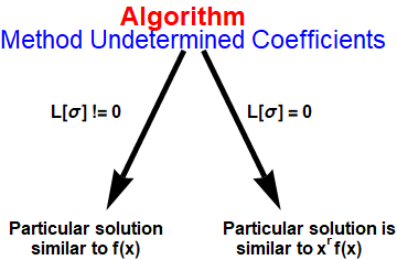
Algorithm of the Method of Undetermined Coefficients
Our main objective is to show how to find a particular solution to
the nonhomogeneous (also called driven or forced) equation
\[
L\left[\texttt{D}\right] y = f(x),
\]
where f(x) is a given function of specific form and L is
a linear constant coefficient differential operator. Since it is assumed that the input function f(x) is annihilated by some constant coefficient linear operator M, we can represent this function as the sum
Therefore, we can restrict ourselves with an input function that is annihilated by one of the above operators.
In this section, we present the algorithm for implementation of the method of undetermined coefficients
that allows one to find a particular solution in case when
the coefficients \( a_n , \ a_{n-1} , \ \ldots , \ a_1 , \ a_0 \) are constants and
f(x) is a constant, a polynomial function, an exponential function eax, a sine or cosine
function \( \sin \beta x \quad \mbox{or}\quad \cos \beta x, \) or finite sums and products
of these functions.
To each of these input functions, called admissible for the method of undetermined coefficients, we assign
a control number, summarized in the table below.
A control number is just a root of the characteristic polynomial that corresponds to the operator annihilating the function. For instance,
if a control number is known to be α, we know that the annihilating polynomial for such function must be
\( \left( \texttt{D} - \alpha \right)^m , \) for some positive integer m (called the multiplicity).
Since the characteristic polynomial for any constant coefficient differential operator can be factored into simple terms,
it is natural to start analyzing with some such simple multiples.
Example:
The following functions all have zero control number:
The above theorem shows that we can always reduce the problem of finding a particular solution to a nonhomogeneous
equation to the case when the input function does not contain an exponential multiple. We illustrate the method of
undetermined coefficients in the series of examples.
Example: Consider the differential equation of third order
with input function \( p(x) = x^3 \) being a polynomial in x. Since the characteristic polynomial
\( L[\lambda ] = \lambda^3 -2\,\lambda^2 -5\,\lambda +6 = \left( \lambda -1 \right) \left( \lambda -2 \right) \left( \lambda -3 \right) \)
has three positive distinct roots while the input function has the control number 0, we seek a particular solution
in the same form as the driven term, namely, as a polynomial of degree 3:
\[
y_p (x) = c_0 + c_1 x + c_2 x^2 + c_3 x^3 ,
\]
where coefficients c's should be determined upon substituting yp into the given differential equation:
Since the driving function \( f(x) = x^3 e^x \) has the control number -1, which does not match
the roots of characteristic equation, the method suggests to seek a particular solution in the same form and the input function:
As we see, practical application of the method of undetermined coefficients requires a lot of calculations; so a
computer algebra is very helpful. To reduce tedious calculations, we apply the formula from the annihilating method:
which we denote by \( M \left[ \texttt{D} \right] = \texttt{D}^3 -5 \texttt{D}^2 + 2 \texttt{D} +8 . \)
Then instead of the original nonhomogeneous problem with the driving term containing exponential multiple, we get
equivalent problem with polynomial right-hand side term:
\[
M \left[ \texttt{D} \right] y = x^3 \qquad \mbox{or} \qquad y''' -5 y'' + 2y' +8y =x^3 .
\]
Since the characteristic polynomial corresponding to the differential operator M has three distinct real roots
\( \lambda = -1, \ 2, \ 4 \) that do not match zero (control number of x3),
we seek its particular solution in the form
\[
y_p (x) = c_0 + c_1 x + c_2 x^2 + c_3 x^3 .
\]
Substituting this function into the differential equation \( y''' -5 y'' + 2y' +8y =x^3 , \)
we obtain exactly the same system of algebraic equations:
We have two options to determine a particular solution: either seek a function having exponential multiple or reduce
the problem to the polynomial input without exponential multiple. We demonstrate both approaches.
The control number of the driving term is σ = 1, which matches one of the roots of the characteristic equation
\( \lambda^3 -2 \lambda^2 -5 \lambda + 6 = \left( \lambda -1 \right) \left( \lambda -2 \right)\left( \lambda -3 \right) =0 \)
of multiplicity 1. Therefore, we seek its particular solution in the form:
\[
y_p (x) = x \left( c_0 + c_1 x + c_2 x^2 + c_3 x^3 \right) e^{x} .
\]
Substituting this function into the given equation and equating coefficients of like powers of x, we obtain the following system of algebraic equations
Now we use Eq.(A) and reduce the problem to the following differential equation:
\[
M\left[ \texttt{D} \right] y \equiv L \left[ \texttt{D} +1 \right] y = x^3 \qquad \Longleftrightarrow \qquad y''' + y'' -6y' = x^3 .
\]
Since the characteristic polynomial \( \lambda^3 + \lambda^2 -6 \lambda = \lambda \left( \lambda -2 \right) \left( \lambda +3 \right) \)
has a root that matches the control number σ = 0 of the input polynomial, we seek its particular solution in the form:
The characteristic polynomial \( L[\lambda ] = \lambda^2 \left( \lambda +2 \right) \left( \lambda -1 \right) \)
has three real roots, one of which, λ = 0, is of multiplicity 2. Since the control number σ = 0 matches
this root, we seek a particular solution in the form of a polynomial of degree 3 multiplied by x2:
The characteristic polynomial \( L[\lambda ] = \left( \lambda -2 \right)^3 \left( \lambda +1 \right) \)
has one triple root λ = 2 and one simple root λ = -1. Since the control number σ = 2 matches this
root, we seek a particular solution as a product of a polynomial of degree 3 times the exponential term, then multiplied
by x3:
Substituting this function into the given differential equation, canceling the exponential multiple and equating like
powers of x, we obtain the following system of algebraic equations:
Example:
Consider the differential equation whose characteristic polynomial has
complex roots that do not match the control numbers of the input function:
\[
L[\texttt{D}] y (x) = \left( \texttt{D}^3 -4\,\texttt{D}^2 +14\,\texttt{D} -20 \right) y \equiv \left( \texttt{D} -2 \right) \left( \texttt{D}^2 -2\texttt{D} +10 \right) y
\equiv y''' -4\,y'' +14\,y' -20\,y
= x \, e^{x}\, \cos 2x .
\]
The characteristic polynomial \( L[\lambda ] = (\lambda -2) \left[ (\lambda -1)^2 + 9 \right] \)
has only simple roots, one is real λ = 2 and two are complex conjugate \( \lambda = 1 \pm 3{\bf j} . \)
The control number of the input function σ = 1 + 2j does not match neither of the roots.
Therefore, we seek a particular solution in the same form as the driving function:
where a0, a1, b0, and b1 are constants to be determined.
Substituting this function into the given differential equation and canceling the exponential term, we obtain
\[
-\left( 5a_0 + 3a_1 -10b_0 + 4b_1 +5a_1 x -10b_1 x \right) \cos 2x - \left( 10a_0 - 4a_1 + 5b_0 + 3b_1 +10 a_1 x + 5b_1 x \right) \sin 2x = x\,\cos 2x .
\]
Example:
Consider the differential equation of second order whose characteristic
polynomial has complex roots that do match the control numbers of the input function:
\[
L[\texttt{D}] y (x) = \left( \texttt{D}^2 +4 \right) y
\equiv y'' +4\,y
= 2\, x^2\, \sin 2x + 3x\, \cos x .
\]
The characteristic polynomial \( L[\lambda ] = \lambda^2 +4 \) has two complex conjugate roots
\( \lambda = \pm 2{\bf j} , \) which matches the control number of the function
\( 2\, x^2\, \sin 2x . \) Another function \( 3x\, \cos x \)
has the control number σ = j (here j is a unit vector in vertical direction on the complex plane, so
\( {\bf j}^2 =-1 \) ). Therefore, we seek a particular solution in the form
\[
y_p (x) = x\left( a_0 + a_1 x + a_2 x^2 \right) \cos 2x + x \left( b_0 + b_1 x + b_2 x^2 \right) \sin 2x
+ \left( c_0 + c_1 x \right) \cos x + \left( c_3 + c_4 x \right) \sin x ,
\]
with some coefficients to be determined. Substituting yp into the differential equation, we obtain
Example:
Consider the differential equation of fourth order whose characteristic
polynomial has complex roots that do match the control numbers of the input function:
\[
L[\texttt{D}] y (x) = \left( \texttt{D}^2 +4 \right)^2 y \equiv \left( \texttt{D}^4 + 8 \texttt{D}^2 +16 \right) y
\equiv y^{(4)} +8\,y'' +16\,y' -y
= 2\, x^2\, \sin 2x + 3x\, \cos x .
\]
Since the input function, \( 2\, x^2\, \sin 2x + 3x\, \cos x , \) is the sum of two functions
of control numbers σ = 2j and σ = j, it is annihilated by the differential operator
\( M\left[ \texttt{D} \right] = \left( \texttt{D}^2 +4 \right)^3 \left( \texttt{D}^2 +1 \right)^2 . \)
Multiplying both sides of the given differential equation by \( M\left[ \texttt{D} \right] , \)
we reduce it to a homogeneous equation
Using the method of undetermined coefficients, find a particular solution to
the differential equation
\( y'' + y = t^2 . \)
Return to Mathematica page
Return to the main page (APMA0330)
Return to the Part 1 (Plotting)
Return to the Part 2 (First Order ODEs)
Return to the Part 3 (Numerical Methods)
Return to the Part 4 (Second and Higher Order ODEs)
Return to the Part 5 (Series and Recurrences)
Return to the Part 6 (Laplace Transform)
Return to the Part 7 (Boundary Value Problems)