Return to computing page for the second course APMA0340
Return to computing page for the fourth course APMA0360
Return to Mathematica tutorial for the first course APMA0330
Return to Mathematica tutorial for the second course APMA0340
Return to Mathematica tutorial for the fourth course APMA0360
Return to the main page for the course APMA0330
Return to the main page for the course APMA0340
Return to the main page for the course APMA0360
Return to Part VI of the course APMA0330
Glossary
Tauberian Theorem:
If f and its derivative are a piecwise continuous functions on [0, ∞) of some exponential order, then its Laplace transform fL satisfies
\begin{equation} \label{EqLaplace.4}
\lim_{\lambda \to \infty} \,\lambda\,f^L (\lambda ) = \lim_{\lambda\to \infty} \,\lambda \int_0^{\infty} f(t)\,e^{-\lambda\,t}\,{\text d}t = \lim_{t\to 0} f(t) = f(0^{+}) .
\end{equation}
\begin{equation} \label{EqLaplace.5}
\lim_{\lambda \to 0} \,\lambda\,f^L (\lambda ) = \lim_{t\to \infty} f(t) .
\end{equation}
Table of Laplace transforms
It is useful to have a “library” of Laplace transforms at hand; some common ones are listed below.
| f(t) | fL(λ) |
|---|---|
| \( \displaystyle e^{at}\,f(t) \) | \( \displaystyle f^L (\lambda - a) \) |
| \( \displaystyle a \,e^{-ab\,t}\, f\left( a\,t \right) \) | \( \displaystyle f^L \left( \frac{\lambda}{a} + b \right) \) |
| \( \displaystyle e^{at} \) | 1/(λ - 𝑎) |
| sin ωt | \( \displaystyle \frac{\omega}{\lambda^2 + \omega^2} \) |
| \( \displaystyle t\,\sin \omega t \) | \( \displaystyle \frac{2\omega\lambda}{\left( \lambda^2 + \omega^2 \right)^2} \) |
| \( \displaystyle e^{kt}\,\sin \omega t \) | \( \displaystyle \frac{\omega}{(\lambda -k )^2 + \omega^2} \) |
| sinh ωt | \( \displaystyle \frac{\omega}{\lambda^2 - \omega^2} \) |
| t sinh ωt | \( \displaystyle \frac{2\,\omega\lambda}{\left( \lambda^2 - \omega^2 \right)^2} \) |
| \( \displaystyle \cos \omega t - \omega t\,\sin \omega t \) | \( \displaystyle \frac{\lambda \left( \lambda^2 - \omega^2 \right)}{\left( \lambda^2 + \omega^2 \right)^2} \) |
| \( \displaystyle \cos \omega t + \omega t\,\sin \omega t \) | \( \displaystyle \frac{\lambda \left( \lambda^2 + 3\,\omega^2 \right)}{\left( \lambda^2 + \omega^2 \right)^2} \) |
| tp | \( \displaystyle \frac{\Gamma (p+1)}{\lambda^{p+1}} \) |
| \( \displaystyle \left( \pi \,t \right)^{-1/2} \) | \( \displaystyle \lambda^{-1/2} \) |
| \( \displaystyle \frac{\sin \omega t}{t} \) | \( \displaystyle \arctan \frac{\omega}{\lambda} \) |
| \( \displaystyle \frac{2}{t} \left( 1 - \cos \omega t \right) \) | \( \displaystyle \ln \left( 1 + \frac{\omega^2}{\lambda^2} \right) \) |
| f(t) | fL(λ) |
|---|---|
| \( \displaystyle f\ast g(t) = \int_0^t f(\tau )\,g(t-\tau )\,{\text d}\tau = g\ast f(t) \) | fLgL |
| H(t) | 1/λ |
| δ(t) | 1 |
| \( \displaystyle t^p\, e^{kt} \) | \( \displaystyle \frac{\Gamma (p+1)}{(\lambda -k)^{p+1}} \) |
| cos ωt | \( \displaystyle \frac{\lambda}{\lambda^{2} + \omega^2} \) |
| t cos ωt | \( \displaystyle \frac{\lambda^2 - \omega^2}{\left( \lambda^{2} + \omega^2 \right)^2} \) |
| \( e^{kt}\cos \omega t \) | \( \displaystyle \frac{\lambda -k}{(\lambda - k)^2 + \omega^2} \) |
| cosh ωt | \( \frac{\lambda}{\lambda^{2} - \omega^2} \) |
| t cosh ωt | \( \frac{\lambda^2 + \omega^2}{\left( \lambda^{2} - \omega^2 \right)^2} \) |
| \( \displaystyle \sin \omega t - \omega t\,\cos \omega t \) | \( \displaystyle \frac{2\,\omega^3}{\left( \lambda^2 + \omega^2 \right)^2} \) |
| \( \displaystyle \sin \omega t + \omega t\,\cos \omega t \) | \( \displaystyle \frac{2\,\omega \lambda^2}{\left( \lambda^2 + \omega^2 \right)^2} \) |
| \( \displaystyle \frac{1}{t} \left( 1 - e^{-t} \right) \) | \( \displaystyle \ln \left( 1 + \frac{1}{\lambda} \right) \) |
| \( \displaystyle \frac{2}{t}\,\sinh at \) | \( \displaystyle \ln \frac{\lambda + a}{\lambda - a} = 2\,\mbox{arctanh} \frac{a}{\lambda} \) |
| \( \displaystyle \frac{2}{t} \left( 1 - \cosh at \right) \) | \( \displaystyle \ln \left( 1 - \frac{a^2}{\lambda^2} \right) \) |
\[
f^L = {\cal L} \left[ f(t) \right] (\lambda ) = \int_0^{\infty} e^{-\lambda\,t}f(t)\,{\text d}t , \qquad \Gamma (\nu ) = \int_0^{\infty} t^{\nu -1} e^{-t} {\text d}t , \qquad H(t) = \begin{cases} 1 , & \ \mbox{ if } t > 0, \\
1/2 , & \ \mbox{ if } t = 0, \\
0, & \ \mbox{ if } t < 0. \end{cases}
\]
The error function erf is defined by
\[
\mbox{erf}(x) = \frac{2}{\sqrt{\pi}} \int_0^x e^{-t^2} {\text d}t .
\]
Its Laplace transform is
\[
{\cal L}_{t\to\lambda} \left[ \mbox{erf}(\sqrt{t}) \right] = \frac{1}{\lambda \sqrt{1+\lambda}} .
\]
Expressions with Bessel and Modified Bessel Functions
| Original function f(t) | Laplace transform fL |
|---|---|
| \( \displaystyle J_0 \left( at \right) \) | \( \displaystyle \frac{1}{\sqrt{\lambda^2 + a^2}} \) |
| \( \displaystyle I_0 \left( at \right) \) | \( \displaystyle \frac{1}{\sqrt{\lambda^2 - a^2}} \) |
| \( \displaystyle J_0 \left( 2\sqrt{at} \right) \) | \( \displaystyle \frac{1}{\lambda}\, e^{-a/\lambda} \) |
| \( \displaystyle I_0 \left( 2\sqrt{at} \right) \) | \( \displaystyle \frac{1}{\lambda}\, e^{a/\lambda} \) |
| \( \displaystyle J_{\nu} \left( at \right) , \qquad \nu > 1\) | \( \displaystyle \frac{a^{\nu}}{\sqrt{\lambda^2 + a^2} \left( \lambda + \sqrt{\lambda^2 + a^2} \right)^{\nu}} \) |
| \( \displaystyle I_{\nu} \left( at \right) , \qquad \nu > 1\) | \( \displaystyle \in \frac{a^{\nu}}{\sqrt{\lambda^2 - a^2} \left( \lambda + \sqrt{\lambda^2 - a^2} \right)^{\nu}} \) |
| \( \displaystyle t^{\nu} J_{\nu} \left( at \right) , \qquad \nu > -\frac{1}{2} \) | \( \displaystyle 2^{\nu} \pi^{-1/2} \Gamma \left( \nu + \frac{1}{2} \right) a^{\nu} \left( \lambda^2 + a^2 \right)^{-\nu -1/2} \) |
| \( \displaystyle t^{\nu} I_{\nu} \left( at \right) \) | \( \displaystyle 2^{\nu} \pi^{-1/2} \Gamma \left( \nu + \frac{1}{2} \right) a^{\nu} \left( \nu^2 - a^2 \right)^{-\nu -1/2} \) |
Elementary Properties of the Laplace Transforms
- Linearity: \( {\cal L} \left[ \alpha\,f(t) + \beta\, g(t) \right] = \alpha\, {\cal L} \left[ f \right]
+ \beta\,{\cal L} \left[ g \right] = \alpha\, f^L + \beta \, g^L . \)
For arbitrary cosnatnts α and β, we have\begin{align*} {\cal L} \left[ \alpha f(t) + \beta g(t) \right] &= \int_0^{\infty} e^{-\lambda t} \left[ \alpha f(t) + \beta g(t) \right] {\text d}t \\ &= \int_0^{\infty}\left[ \alpha f(t)\, e^{-\lambda t} + \beta g(t)\, e^{-\lambda t} \right] {\text d}t \\ &= \int_0^{\infty}\alpha f(t)\, e^{-\lambda t} {\text d}t + \int_0^{\infty} \beta g(t) \, e^{-\lambda t} {\text d}t \\ &= \alpha \int_0^{\infty} f(t)\, e^{-\lambda t} {\text d}t + \beta \int_0^{\infty} g(t) \, e^{-\lambda t} {\text d}t \\ &= \alpha {\cal L} \left[ f(t) \right] + \beta {\cal L} \left[ g(t) \right] = \alpha\,f^L + \beta \,g^L . \end{align*}
- The derivative rule:
\begin{equation} \label{EqTable.2} {\cal L} \left[ f^{(n)} (t) \right] = \lambda^n - \sum_{k=1}^n \lambda^{n-k} f^{(k-1)} (+0) . \end{equation}In particular,\begin{equation} \label{EqTable.3} {\cal L} \left[ f' (t) \right] = {\cal L} \left[ \frac{{\text d}f (t)}{{\text d}t} \right] = \lambda\,f^L (\lambda ) - f(+0) . \end{equation}\begin{equation} \label{EqTable.4} {\cal L} \left[ f'' (t) \right] = {\cal L} \left[ \frac{{\text d}^2 f (t)}{{\text d}t^2} \right] = \lambda^2 f^L (\lambda ) - f'(+0) - \lambda\,f(+0) . \end{equation}By mathematical induction, utilizing integration by parts\[ {\cal L} \left[ f' (t) \right] = \int_0^{\infty} e^{-\lambda t} f' (t)\, {\text d}t = \left. e^{-\lambda t} f (t) \right\vert_{t=0}^{t=\infty} - \lambda \int_0^{\infty} e^{-\lambda t} f (t)\, {\text d}t = -f(+0) + \lambda\,f^L (\lambda ) . \] Assuming the property holds for n = k ∈ ℤ+, we have\[ {\cal L} \left[ f^{(k)} (t) \right] = \lambda^k f^L - \lambda^{k-1} f(+0) - \lambda^{k-2} f' (+0) - \cdots - \lambda\,f^{(k-2)} (+0) - f^{(k-1)} (+0) . \]We now prove for n = k + 1.\begin{align*} {\cal L} \left[ f^{(k+1)}(t) \right] &= \int_0^{\infty} e^{-\lambda t} f^{(k+1)}(t) \,{\text d}t = \lim_{A\to \infty} \int_0^A e^{-\lambda t} f^{(k+1)}(t) \,{\text d}t \\ &= \lim_{A\to \infty} \left[ \left. e^{-\lambda t} f^{(k)}(t) \right\vert_{t=0}^{t=A} + \lambda \int_0^A f^{(k)}(t) e^{-\lambda t} {\text d}t \right] \\ &= \lambda\,{\cal L} \left[ f^{(k)}(t) \right] - f^{(k)}(+0) \end{align*}and the statement follows.
- Convolution rule: \( {\cal L} \left[ f \ast g \right] = f^L \,g^L . \)
Recall that the convolution of two functions f and g is\begin{equation} \label{EqTable.1} \left( f \ast g \right) (t) = \int_0^t f(t-\tau )\,g(\tau ) \,{\text d} \tau = \int_0^t g(t-\tau )\,f(\tau ) \,{\text d} \tau = \left( g \ast f\right) (t) . \end{equation}Application of the Laplace transformation to the convolution integral \eqref{EqTable.1} yields\[ {\cal L} \left[ f*g \right] (\lambda ) = \int_0^{\infty} e^{-\lambda t} {\text d} t \int_0^{t} f(\tau )\, g(t-\tau )\, {\text d}\tau . \]Reversing the order of integration gives\[ {\cal L} \left[ f*g \right] (\lambda ) = \int_0^{\infty} {\text d}\tau .f(\tau ) \, e^{-\lambda \tau} \int_{\tau}^{\infty} {\text d} t\,g(t-\tau )\, e^{-\lambda (t- \tau )} \]Substitution u = −τ shows that\[ {\cal L} \left[ f*g \right] (\lambda ) = \int_0^{\infty} {\text d}\tau .f(\tau ) \, e^{-\lambda \tau} \int_{0}^{\infty} {\text d} u\, g(u) \, e^{-\lambda u} = f^L \cdot g^L . \]To finish the proof, we need to show that the convolution is a function-original.- Shift rule: \( {\cal L} \left[ f(t-a)\,H(t-a) \right] = e^{-a\lambda} \,f^L (\lambda ) . \)
\begin{align*} {\cal L} \left[ H(t-a)\,f(t-a) \right] &= \int_0^{\infty} e^{-\lambda t} H(t-a)\,f(t-a)\, {\text d} t = \int_a^{\infty} e^{-\lambda t}\,f(t-a)\, {\text d} t \\ &= \int_0^{\infty} e^{-\lambda \left( \tau + a \right)} f\left( \tau \right) {\text d} \tau \end{align*}because of substitution t = τ + 𝑎. Then\[ {\cal L} \left[ H(t-a)\,f(t-a) \right] = \int_0^{\infty} e^{-\lambda \left( \tau + a \right)} f\left( \tau \right) {\text d} \tau = e^{-\lambda a} f^L (\lambda ) . \]- Similarity rule: \( {\cal L} \left[ f(kt) \right] = \frac{1}{k}\, f^L \left( \frac{\lambda}{k} \right) . \)
\begin{align*} {\cal L} \left[ f(kt) \right] &= \int_0^{\infty} e^{-\lambda t} f(kt)\,{\text d}t = \frac{1}{k} \int_0^{\infty} e^{-\lambda u/k} f(u)\,{\text d}u \\ &= \frac{1}{k} \, f^L \left( \frac{\lambda}{k} \right) . \end{align*}- Attenuation rule: \( {\cal L} \left[ e^{-at} \, f(t) \right] = f^L \left( \lambda +a \right) . \)
\[ {\cal L} \left[ e^{-at} \, f(t) \right] = \int_0^{\infty} e^{-at} e^{-\lambda t} f(t)\, {\text d}t = \int_0^{\infty} e^{-at - \lambda t} f(t)\, {\text d}t = f^L (\lambda + a ) . \]- Differentiation rule: \( \frac{{\text d}}{{\text d} \lambda} \, f^L (\lambda ) = - {\cal L} \left[ t\, f(t) \right] . \) In deneral, for a positive integer n,
\[ {\cal L} \left[ t^n f(t) \right] = \left( -1 \right)^n \frac{{\text d}^n}{{\text d}\lambda^n} \,{\cal L} \left[ f(t) \right] = \left( -1 \right)^n \frac{{\text d}^n}{{\text d}\lambda^n} \,f^L (\lambda ) . \]Using mathematical induction,\[ {\cal L} \left[ t\, f(t) \right] = \int_0^{\infty} t\,f(t)\,e^{-\lambda t} {\text d}t = - \int_0^{\infty} f(t)\,\frac{\text d}{{\text d}\lambda}\,e^{-\lambda t} {\text d}t = -\frac{\text d}{{\text d}\lambda} \int_0^{\infty} f(t)\,e^{-\lambda t} {\text d}t = - \frac{\text d}{{\text d}\lambda} \,f^L (\lambda ) . \]Assuming that the property holds for n = k ∈ ℤ+, then\[ {\cal L} \left[ t^k f(t) \right] = \left( -1 \right)^k \frac{{\text d}^k}{{\text d}\lambda^k} \,{\cal L} \left[ f(t) \right] = \left( -1 \right)^k \frac{{\text d}^n}{{\text d}\lambda^k} \,f^L (\lambda ) . \]We now prove that the property holds for n = k+1,\begin{align*} \left( -1 \right)^{k+1} \frac{{\text d}^{k+1}}{{\text d}\lambda^{k+1}}\, f^L (\lambda ) &= \left( -1 \right) \left( -1 \right)^k \frac{{\text d}}{{\text d}\lambda} \left[ \frac{{\text d}^{k}}{{\text d}\lambda^{k}}\, f^L (\lambda ) \right] \\ &\quad \\ &= \left( -1 \right) \frac{{\text d}}{{\text d}\lambda} \left[ \left( -1 \right)^k \frac{{\text d}^{k}}{{\text d}\lambda^{k}}\, f^L (\lambda ) \right] = \left( -1 \right) \frac{{\text d}}{{\text d}\lambda} \,{\cal L} \left[ t^k f(t) \right] \\ &\quad \\ &= \left( -1 \right) \frac{{\text d}}{{\text d}\lambda} \int_0^{\infty} \left[ t^k f(t) \, e^{-\lambda t} \right] {\text d} t \\ &\quad \\ &= \int_0^{\infty} \frac{\partial}{\partial \lambda} \left[ t^k f(t)\, e^{-\lambda t} \right] {\text d} t \\ &\quad \\ &= \int_0^{\infty} e^{-\lambda t} t^{k+1} f(t) \, {\text d} t = {\cal L} \left[ t^{k+1} f(t) \right] . \end{align*}- Integration rule: \( {\cal L} \left[ t^n \ast f(t) \right] = \frac{n!}{\lambda^{n+1}} \, f^L (\lambda ) . \)
In particular, for n = 0,\[ {\cal L} \left[ \int_0^t f(s)\,{\text d}s \right] = \frac{1}{\lambda}\, f^L (\lambda ) . \]The property follows from the convolution rule.- The Laplace transform of periodic functions.
If \( f(t) = f(t+ \omega ) , \) then \( \displaystyle f^L (\lambda ) = \int_0^{\infty} f(t )\,e^{-\lambda\,t} \,{\text d} t = \frac{1}{1- e^{-\omega\lambda}} \, \int_0^{\omega} \,f(t ) \,e^{-\lambda \, t} \,{\text d} t . \)If f(t) is periodic with period ω and its Laplace transform exists, then\begin{align*} f^L (\lambda ) &= {\cal L} \left[ f(t) \right] = \int_0^{\infty} e^{-\lambda t} f(t)\, {\text d}t \\ &= \int_0^{\omega} e^{-\lambda t} f(t)\, {\text d}t + \int_{\omega}^{\infty} e^{-\lambda t} f(t)\, {\text d}t \qquad \mbox{make substitution at the latter} \\ &= \int_0^{\omega} e^{-\lambda t} f(t)\, {\text d}t + \int_0^{\infty} e^{-\lambda (u+\omega )} f(u + \omega )\, {\text d}u \\ &= \int_0^{\omega} e^{-\lambda t} f(t)\, {\text d}t + e^{-\lambda\omega} \int_0^{\infty} e^{-\lambda u} f(u)\, {\text d}u \\ &= \int_0^{\omega} e^{-\lambda t} f(t)\, {\text d}t + e^{-\lambda\omega} f^L . \end{align*}The required identity follows from the equation\[ f^L = \int_0^{\omega} e^{-\lambda t} f(t)\, {\text d}t + e^{-\lambda\omega} f^L . \]- The Laplace transform of anti-periodic functions.
If \( f(t) = -f(t+ \omega ) , \) then \( \displaystyle f^L (\lambda ) = \int_0^{\infty} f(t )\,e^{-\lambda\,t} \,{\text d} t = \frac{1}{1+ e^{-\omega\lambda}} \, \int_0^{\omega} \,f(t ) \,e^{-\lambda \, t} \,{\text d} t . \)Proof is similar to the previous one.- Division by t:
\( \displaystyle {\cal L} \left[ \frac{f(t)}{t} \right] (\lambda ) = \int_{\lambda}^{\infty} f^L (u)\,{\text d}u . \)\begin{align*} \int_{\lambda}^{\infty} f^L (s)\,{\text d}s &= \int_{\lambda}^{\infty} {\text d}s \int_0^{\infty} e^{-st} f(t) \,{\text d}t \\ &= \int_0^{\infty} {\text d}t \int_{\lambda}^{\infty} e^{-st} f (s)\,{\text d}s \\ &= \int_0^{\infty} {\text d}t\left[ \lim_{k\to\infty} \int_{\lambda}^{k} e^{-st} f (s)\,{\text d}s \right] \\ &= \int_0^{\infty} {\text d}t\left[ \lim_{k\to\infty} \left. f(t) \,\frac{e^{-st}}{-t} \right\vert_{s}^k \right] = \int_0^{\infty} {\text d}t \lim_{k\to\infty} \left[ e^{-st} - e^{-kt} \right] \frac{f(t)}{t} \\ &= {\cal L} \left[ \frac{1}{t}\, f(t) \right] . \end{align*}Table of Laplace transform properties in Mathematica:
nvlpltList = {1, E^(a t), t^2, t^p, Sqrt[t], t^(n - 1/2), Sin[a t], Cos[a t], t Sin[a t], t Cos[a t](*#10*), Sin[a t] - a t Cos[a t], Sin[a t] + a t Cos[a t], Cos[a t] - a t Sin[a t], Cos[a t] + a t Sin[a t], Sin[a t + b], Cos[a t + b], Sinh[a t], Cosh[a t], E^(a t) Sin[b t], E^(a t) Cos[b t](*#20*), E^(a t) Sinh[b t], E^(a t) Cosh[b t], t^n E^(a t), f[c t], HeavisideTheta[t], DiracDelta[t - 1], HeavisideTheta[t] f[t - c], HeavisideTheta[t] g[t], E^(c t) f[t], t^n f[t](*#30*), 1/t f[t], \!\( \*SubsuperscriptBox[\(\[Integral]\), \(0\), \(t\)]\(f[ v] \[DifferentialD]v\)\), \!\( \*SubsuperscriptBox[\(\[Integral]\), \(0\), \(t\)]\(f[ t - \[Tau]]\ g[\[Tau]] \[DifferentialD]\[Tau]\)\), f[t + T], f'[t], f''[t], (f^(n))[t]}; lpltList = LaplaceTransform[#, t, s] & /@ invlpltList // FullSimplify; TableForm[ Table[{i, invlpltList[[i]], lpltList[[i]]}, {i, 1, Length[lpltList]}]]Definition: The full-wave rectifier of a function f(t), defined on a finite interval 0≤t≤T, is a periodic function with period T that is equal to f(t) on the interval [0,T].
The half-wave rectifier of a function f(t), defined on a finite interval 0≤t≤T, is a periodic function with period 2T that coincides with f(t) on the interval [0,T] and is identically zero on the interval [T,2T].half = Plot[f[t], {t, 0, 4*Pi}, PlotStyle -> Thickness[0.015], AspectRatio -> 1, Axes -> False];
txt = Graphics[Text[Style["f(t)", FontSize -> 14, Red], {1.5, 0.3}]];
t0 = Graphics[Text[Style["0", FontSize -> 14, Black], {-0.1, -0.5}]];
t1 = Graphics[Text[Style["T", FontSize -> 14, Black], {3.1, -0.5}]];
t2 = Graphics[Text[Style["2T", FontSize -> 14, Black], {6.3, -0.5}]];
t3 = Graphics[Text[Style["3T", FontSize -> 14, Black], {9.35, -0.5}]];
txt2 = Graphics[Text[Style["f(t)", FontSize -> 14, Red], {7.8, 0.3}]];
Show[txt, half, t0, t1, t2, t3, txt2]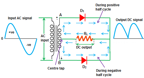
Full-wave rectifier. 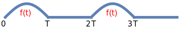
Half-wave rectifier. Example 1: Consider a linear function f(t) = t on the interval [0, ∞). For a positive T, its full-wave rectifier is\[ g(t) = t \left[ H(t) - H(t-T) \right] + \left( t-T \right) \left[ H(t-T) - H(t-2T) \right] + \left( t-2T \right) \left[ H(t-2T) - H(t-3T) \right] + \cdots . \]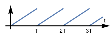
We plot full wave rectifier of function f(t) = t: f[t_] = Piecewise[{{t, 0 < t < 1}, {t-1, 1 < t < 2}, {t - 2, 2 < t < 3}, {t-3, 3 < t < 4}, {t - 4, 4 < t < 5}}];
plot = Plot[f[t], {t, 0, 3.5}, PlotStyle -> Thickness[0.01], AspectRatio -> 1/3, Axes -> False, PlotRange -> {{-0.4, 3.8}, {-0.6, 1.5}}];
ar = Graphics[{Black, Thickness[0.01], Arrowheads[0.08], Arrow[{{-0.2, 0}, {3.8, 0}}]}];
ar2 = Graphics[{Black, Thickness[0.01], Arrowheads[0.08], Arrow[{{0, -0.2}, {0, 1.2}}]}];
tt = Graphics[{Black, Text[Style["t", 18], {3.6, 0.3}]}];
t1 = Graphics[{Black, Text[Style["T", 18], {1, -0.3}]}];
t2 = Graphics[{Black, Text[Style["2T", 18], {2, -0.3}]}];
t3 = Graphics[{Black, Text[Style["3T", 18], {3, -0.3}]}];
Show[plot, ar, ar2, tt, t1, t2, t3]Full-wave rectifier of function f = t. Mathematica code
Since the full wave rectifier is a periodic function with period T, its Laplace transform is\[ {\cal L} \left[ g(t) \right] = \frac{1}{1 - e^{-\lambda T}} \, \int_0^T t\,e^{-\lambda t} {\text d}t = \frac{1}{\lambda^2} - \frac{T}{1 - e^{-\lambda T}} \,\frac{1}{\lambda} \,e^{-\lambda T} . \]Assuming[ ss > 0, Integrate[t*Exp[-ss*t], {t, 0, TT}]](1 - E^(-ss TT) (1 + ss TT))/ss^2
Now we consider the half-wave rectifier that corresponds to the linear function. It is a 2T periodic function:\[ h(t) = t \left[ H(t) - H(t-T) \right] + \left( t-2T \right) \left[ H(t-2T) - H(t-3T) \right] + \left( t-4T \right) \left[ H(t-4T) - H(t-5T) \right] + \cdots . \]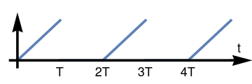
We plot full wave rectifier of function f(t) = t: f[t_] = Piecewise[{{t, 0 < t < 1}, {0, 1 < t < 2}, {t - 2, 2 < t < 3}, {0, 3 < t < 4}, {t - 4, 4 < t < 5}}];
plot = Plot[f[t], {t, 0, 5.3}, PlotStyle -> Thickness[0.01], AspectRatio -> 1/3, Axes -> False, PlotRange -> {{-0.4, 5.5}, {-0.6, 1.5}}];
ar = Graphics[{Black, Thickness[0.01], Arrowheads[0.08], Arrow[{{-0.2, 0}, {5.5, 0}}]}];
ar2 = Graphics[{Black, Thickness[0.01], Arrowheads[0.08], Arrow[{{0, -0.2}, {0, 1.2}}]}];
tt = Graphics[{Black, Text[Style["t", 18], {5.2, 0.3}]}];
t1 = Graphics[{Black, Text[Style["T", 18], {1, -0.3}]}];
t2 = Graphics[{Black, Text[Style["2T", 18], {2, -0.3}]}];
t3 = Graphics[{Black, Text[Style["3T", 18], {3, -0.3}]}];
t4 = Graphics[{Black, Text[Style["4T", 18], {4, -0.3}]}];
Show[plot, ar, ar2, tt, t1, t2, t3, t4]Half-wave rectifier of function f = t. Mathematica code
Again, using rule 9, we obtain the Laplace transform of the half-wave rectifier:\[ {\cal L} \left[ h(t) \right] = \frac{1}{1 - e^{-2\lambda T}} \, \int_0^T t\,e^{-\lambda t} {\text d}t = \frac{1}{1 - e^{-2\lambda T}} \,\frac{1}{\lambda^2} \left( 1 - e^{-\lambda T} \right) \left( 1 + \lambda T \right) = \frac{1}{1 + e^{-\lambda T}} \,\frac{1}{\lambda^2} \left( 1 + \lambda T \right) . \]■Example 2: The sine integral function is defined by\[ \mbox{Si}(x) = \int_0^x \frac{\sin t}{t}\,{\text d}t . \]We know that the Laplace transform of the sine function is \( {\cal L} \left[ \sin t \right] = (\lambda^2 + 1)^{-1} . \) Integrating, we obtain according to rule 11 that\[ \int_0^{\infty} e^{-\lambda t} \frac{\sin t}{t}\,{\text d}t = \int_{\lambda}^{\infty} {\cal L} \left[ \sin t \right] (p)\,{\text d}p = \left[ \arctan \lambda \right]_{p = \lambda}^{\lambda = \infty} = \frac{\pi}{2} - \arctan \lambda \]because \( \int \frac{{\text d}t}{t^2 +1} = \arctan t . \) Now we have\begin{align*} {\cal L} \left[ \mbox{Si}(t) \right] &= \int_0^{\infty} e^{-\lambda t} {\text d}t \left( \int_0^t \frac{\sin x}{x}\,{\text d}x \right) = \left[ \frac{e^{-\lambda t}}{-\lambda} \,\int_0^t \frac{\sin x}{x}\,{\text d}x\right]_{t=0}^{\infty} + \frac{1}{\lambda} \int_0^t e^{-\lambda t} \frac{\sin t}{t}\,{\text d}t \\ &= \frac{1}{\lambda} \left( \frac{\pi}{2} - \arctan \lambda \right) = \frac{1}{\lambda} \,\mbox{arccot}(\lambda ) , \qquad \Re\lambda > 1. \end{align*}We check with MathematicaSimplify[LaplaceTransform[SinIntegral[t], t, s]]Unfortunately, Mathematica does not know how to present the answer in an accurate way. ■Example 3: Consider the scaled complementary error function\[ f(t) = \mbox{erfc}\left( \frac{a}{\sqrt{t}} \right) = \frac{2}{\sqrt{\pi}} \,\int_{a/\sqrt{t}}^{\infty} e^{-x^2} {\text d}x = 1 - \mbox{erf} \left( \frac{a}{\sqrt{t}} \right) = 1 - \frac{2}{\sqrt{\pi}} \,\int_{0}^{a/\sqrt{t}} e^{-x^2} {\text d}x , \]where 𝑎 is a positive number. We denote its Laplace transform by F(p), so\begin{align*} F(p) &= {\cal L}_{t\to p} \left[ f(t) \right] = \frac{2}{\sqrt{\pi}} \int_0^{\infty} e^{-pt} {\text d}t \left( \int_{a/\sqrt{t}}^{\infty} e^{-x^2} {\text d}x \right) \\ &= \frac{2}{\sqrt{\pi}} \left( \frac{e^{-pt}}{-p} \left[ \int_{a/\sqrt{t}}^{\infty} e^{-x^2} {\text d}x \right]_{t=0}^{\infty} + \frac{1}{p} \,\int_0^{\infty} {\text d}t \,e^{-pt} \left( - e^{- a^2 /t} \right) \left( - \frac{a}{2}\, \frac{{\text d}t}{t^{/2}} \right) \right) \\ &= \frac{a}{p} \,\frac{1}{\sqrt{\pi}} \int_0^{\infty} e^{-pt-a^2 /t} \frac{{\text d}t}{t^{3/2}} \\ &= \frac{2a}{p\sqrt{\pi}} \int_0^{\infty} e^{-p/x^2 - (ax)^2} {\text d}x \qquad\mbox{where} \quad \frac{1}{\sqrt{t}} = x. \end{align*}To evaluate this integral, let us denote p = b². We introduce an auxiliary integral:\[ I(a,b) = \int_0^{\infty} e^{-b^2/x^2 - (ax)^2} {\text d}x , \]so \( I(a, 0) = \sqrt{\pi} /(2a) . \) Then\[ F(p) = F \left( b^2 \right) = \frac{2a}{p\sqrt{\pi}} \, I(a,b) . \]Substitution 𝑎x = u yields\[ I(a,b) = \frac{1}{b} \int_0^{\infty} e^{-u^2 - a^2 b^2 /u^2} {\text d}u . \]Also\[ \frac{\text d}{{\text d}b} \,I(a,b) = -2b \int_0^{\infty} e^{-u^2 - a^2 b^2 /u^2} \frac{{\text d}u}{u^2} = -2 \int_0^{\infty} e^{-z^2 -a^2 b^2 /z^2} {\text d}z, \qquad z= \frac{b}{x} . \]Thus,\[ \frac{\text d}{{\text d}b} \,I(a,b) = -2a\,I (a,b) \qquad \Longrightarrow \qquad I(a,b) = \frac{\sqrt{\pi}}{2a} \,e^{-2ab} . \]Therefore,\[ F(p) = {\cal L}_{t\to p} \left[ \mbox{erfc}\left( \frac{a}{\sqrt{t}} \right) \right] = \frac{1}{p} \, e^{-2a\sqrt{p}} , \qquad \Re p > 0. \]■Example 4: The cosine integral function is\[ \mbox{Ci}(t) = \int_{\infty}^t \frac{\cos x}{x} \,{\text d}x = - \int_t^{\infty} \frac{\cos x}{x} \,{\text d}x . \]Let f(t) = Ci(t). Since its derivative is\[ \mbox{Ci}'(t) = f' (t) =\frac{\cos t}{t} , \]we find its Laplace transform to be\[ {\cal L}_{t\to p} \left[ t\,f'(t) \right] = {\cal L}_{t\to p} \left[ \cos t\right] = \frac{p}{p^2 +1} . \]Using the derivative rule, we get\[ \frac{\text d}{{\text d}p} \int_0^{\infty} e^{-pt} f' (t) \,{\text d}t = \frac{p}{p^2 +1} . \]This gives\[ \frac{\text d}{{\text d}p} \left[ -f(0) + p\,F(p) \right] = \frac{p}{p^2 +1} . \]Integration yields\[ p\,F(p) = p\,{\cal L}_{t\to p} \left[ f(t) \right] = p\,{\cal L}_{t\to p} \left[ \mbox{Ci}(t) \right] = \frac{1}{2}\,\ln \left( 1 + p^2 \right) + c , \]where c is a constant of integration, which we determine using the Tauberian theorem\[ \lim_{p\to 0} p\,F(p) = \lim_{t\to \infty} f(t) = c = 0. \]■Return to Mathematica page
Return to the main page (APMA0330)
Return to the Part 1 (Plotting)
Return to the Part 2 (First Order ODEs)
Return to the Part 3 (Numerical Methods)
Return to the Part 4 (Second and Higher Order ODEs)
Return to the Part 5 (Series and Recurrences)
Return to the Part 6 (Laplace Transform)
Return to the Part 7 (Boundary Value Problems) - Convolution rule: \( {\cal L} \left[ f \ast g \right] = f^L \,g^L . \)