Preface
This section is devoted for solving first order ODEs with the aid of standard
Mathematica command: DSolve.
Return to computing page for the second course APMA0340
Return to Mathematica tutorial for the first course APMA0330
Return to Mathematica tutorial for the second course APMA0340
Return to the main page for the course APMA0330
Return to the main page for the course APMA0340
Glossary
Solving First Order ODEs
The Wolfram Language function DSolve finds symbolic solutions (that can be expressed implicitly or even explicitly) to certain classes of differential equations. The Wolfram Language function NDSolve, on the other hand, is a general numerical differential equation solver (it is discussed in more details in Part III). DSolve can handle the following types of equations:
- Ordinary Differential Equations (ODEs), in which there are two or more independent variables and one dependent variable. Finding exact symbolic solutions (expressed through elementary and special functions) of ODEs is a difficult problem, but DSolve can solve many first-order ODEs and a limited number of the second-order ODEs found in standard reference books.
- Partial Differential Equations (PDEs), in which there are two or more independent variables and one dependent variable. Finding exact symbolic solutions of PDEs is a difficult problem, but DSolve can solve most first-order PDEs and a limited number of the second-order PDEs found in standard reference books.
- Differential Algebraic Equations (DAEs), in which some members of the system are differential equations and the others are purely algebraic, having no derivatives in them. As with PDEs, it is difficult to find exact solutions to DAEs, but DSolve can solve many examples of such systems that occur in applications. DSolve
DSolve returns results as lists of rules. This makes it possible to return multiple solutions to an equation. A user can utilize the rules to substitute the solutions into other calculations. DSolve finds the general solution for the given ODE. A rule for the function that satisfies the equation is returned.
Let’s look at the first order differential equation \( {\text d}y/{\text d}x=y(x) \) that defined an exponential function as its solution. Indeed, once we enter
You can pin down a specific solution by using the Mathematica command /. (ReplaceAll). This means that Mathematica assigns y[x] to be the general solution (because it contains an arbitrary constant) to the given differential equation.
BesselJ[-(4/5), 2/5 I x^(5/2)] Gamma[1/5] + (-1)^(7/10) 5^(
3/5) x^(5/2) BesselJ[-(6/5), 2/5 I x^(5/2)] Gamma[4/5] + (-1)^(
1/5) 5^(3/5) BesselJ[-(1/5), 2/5 I x^(5/2)] Gamma[4/5] - (-1)^( 7/10) 5^(3/5) x^(5/2)
BesselJ[4/5, 2/5 I x^(5/2)] Gamma[4/ 5])/(2 x (BesselJ[1/5, 2/5 I x^(5/2)] Gamma[1/5] + (-1)^(1/5)
5^(3/5) BesselJ[-(1/5), 2/5 I x^(5/2)] Gamma[4/5]))}}
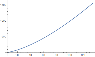
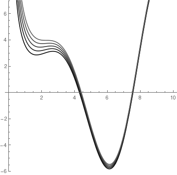
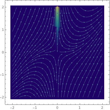
A plot of the solution given by DSolve can give useful information about the nature of the solution, for instance, whether it is oscillatory in nature. It can also serve as a means of solution verification if the shape of the graph is known from theory or from plotting the vector field associated with the differential equation. The solution can be plotted for specific values of the constant C[1] using Plot. The use of Evaluate reduces the time taken by Plot and can also help in cases where the solution has discontinuities.
To get a function as output form DSolve, type
Another possibility to define a function is to use DifferentialRoot[] instead:
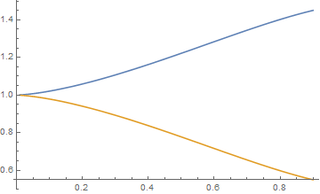
When a differential equation is given in not a normal form, then the equation may have two solutions that can be plotted on the same graph.
{ y -> Function[{x}, 1/5 ( 5 - 2 x^(3/2) Sqrt[1-x^2] - 4 EllipticE[ArcSin[Sqrt[x]], -1] + 4 EllipticF[ArcSin[Sqrt[x]], -1])]}}
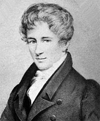
Niels Henrik Abel (1802--1829) was a Norwegian mathematician who made pioneering contributions in a variety of fields. An Abel equation of the first kind, named after Niels Abel, is any ordinary differential equation that is cubic in the unknown function:
where \( f_3 (x) \ne 0 . \) If \( f_3 (x) \equiv 0 , \) then the Abel equation reduces to either Bernoulli equation or to Riccati equation. Associated with any Abel ordinary differential equation (ODE for short) is a sequence of expressions that is built from the coefficients of the equation { f0, f1, f2, f3 } and invariant under certain coordinate transformations of the independent variable and the dependent variable. These invariants characterize each equation and can be used for identifying integrable classes of Abel ODEs. In particular, Abel ODEs with zero or constant invariants can be integrated easily and constitute an important integrable class of these equations.
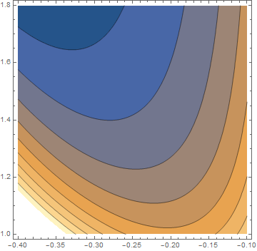
When one tries to solve an Abel equation using Mathematica, the answer could be given in an implicit form.
ContourPlot[expr, {x, -0.4, -0.1}, {y, 1.0, 1.8}]
The design of DSolve is modular: the algorithms for different classes of problems work independently of one another. Once a problem has been classified, the available methods for that class are tried in a specific sequence until a solution is obtained. The code has a hierarchical structure whereby the solution of complex problems is reduced to the solution of relatively simpler problems, for which a greater variety of methods is available. For example, higher-order ODEs are typically solved by reducing their order to 1 or 2.
While differential equations have three basic types---ordinary (ODEs), partial (PDEs), or differential-algebraic (DAEs), they can be further described by attributes such as order, linearity, and degree. The solution method used by DSolve and the nature of the solutions depend heavily on the class of equation being solved.
The order of a differential equation is the order of the highest derivative in the equation. In this part of tutorial, we consider only first-order differential equations that contain a derivative of unknown function.
A differential equation is linear if the equation is of the first degree in y and its derivatives, and if the coefficients are functions of the independent variable. For instance, the differential equation
There is a close relationship between functions and differential equations. Starting with a function of almost any type, it is possible to construct a differential equation satisfied by that function. Conversely, any differential equation gives rise to one or more functions, in the form of solutions to that equation. In almost all cases, there is no better way to define these functions as to say that they are solutions to some differential equations. Generally speaking, it is impossible to represent a solution to a differential equation through elementary functions. In fact, many special functions from classical analysis have their origins in the solution of differential equations. Mathieu functions are one such class of special functions that were discovered in 1868 by him. Émile Léonard Mathieu (1835--1890) was a French mathematician. He is most famous for his work in group theory and mathematical physics. He has given his name to the Mathieu functions, Mathieu groups and Mathieu transformation. He authored a treatise of mathematical physics in 6 volumes. Mathieu was interested in studying the vibrations of elliptical membranes. The eigenfunctions for the wave equation that describes this motion are given by products of Mathieu functions. Mathematica uses two abbreviations for Mathieu functions: MathieuC[a, q, z] for even functions with characteristic value a and parameter q, as well as MathieuS[a, q, z] for odd functions.
There are four major areas in the study of ordinary differential equations that are of interest in
pure and applied science.
- Exact solutions, which are closed-form or implicit analytical expressions that satisfy the given problem.
- Numerical solutions, which are available for a wider class of problems, but are typically only valid over a limited range of the independent variables.
- Qualitative theory, which is concerned with the global properties of solutions and is particularly important in the modern approach to dynamical systems.
- Existence and uniqueness theorems, which guarantee that there are solutions with certain desirable properties provided a set of conditions is fulfilled by the differential equation.
| Name of equation | general form | date | mathematician |
|---|---|---|---|
| Separable | \( y' = p(x)\,q(y) \) | 1691 | Gottfried Leibniz |
| Homogeneous slope | \( y' = f \left( y(x) /x \right) \) | 1691 | Gottfried Leibniz |
| Linear | \( y' = a(x)\,y + f(x) \) | 1694 | Gottfried Leibniz |
| Bernoulli | \( y' = g(x)\, y + h(x)\, y^2 \) | 1695 | James (Jacob) Bernoulli |
| Riccati | \( y' = f(x) + g(x)\, y + h(x)\, y^2 \) | 1724 | Count Riccati |
| Exact | \( M\,{\text d}x + N\,{\text d}y =0 \) with \( M_y = N_x \) | 1734 | Leonhard Euler |
| Clairaut | \( y(x) = x\,y' + f(y' ) \) | 1734 | Alexis Clairaut |
| Abel | \( y' = f_0 (x) + f_1 (x)\,y + f_2 (x)\,y^2 + f_3 (x)\, y^3 \) | 1834 | Niels H. Abel |
| Chini | \( y' = f(x) + g(x)\,y + h(x)\,y^n \) | 1924 | Mineo Chini |
|
gensol = DSolve[x*y'[x] + y[x] == x^2 *Sin[x], y[x], x]
top = Table[gensol[[1, 1, 2]] /. C[1] -> i, {i, 1.37, 4, Pi/5.9}] gray = Table[GrayLevel[i], {i, 0, 0.8, 0.8/9}] Plot[Evaluate[top], {x, 0, 10}, PlotRange -> {-6, 7}, AspectRatio -> 1, PlotStyle -> gray] StreamDensityPlot[{1, x*Sin[x] - y/x}, {x, -2, 2}, {y, -2, 2}, ColorFunction -> "BlueGreenYellow"] |
 |
 |
Return to Mathematica page
Return to the main page (APMA0330)
Return to the Part 1 (Plotting)
Return to the Part 2 (First Order ODEs)
Return to the Part 3 (Numerical Methods)
Return to the Part 4 (Second and Higher Order ODEs)
Return to the Part 5 (Series and Recurrences)
Return to the Part 6 (Laplace Transform)
Return to the Part 7 (Boundary Value Problems)