Return to computing page for the first course APMA0330
Return to computing page for the second course APMA0340
Return to Mathematica tutorial for the first course APMA0330
Return to Mathematica tutorial for the second course APMA0340
Return to the main page for the course APMA0330
Return to the main page for the course APMA0340
Return to Part IV of the course APMA0330
Sometimes higher order differential equations can be reduced to lower and first order equations. We consider two
classes of equations when this is possible.
Dependent Variable Missing
For a differential equation of the form \( y^{(n)} = f(x, y^{(n-1)} ) , \)
the substitution \( p = y^{(n-1)} , \ p' = y^{(n)} \) leads to a first order
equation of the form \( p' = f(x,p) . \) If this equation can be solved for
p, then y can be obtained by integrating
\( {\text d}^{n-1} y/{\text d}x^{n-1} = p . \) Note that one arbitrary constant
is obtained in solving the first order equation for p, and n-1 constants are introduced
in the integration for y.
Example: Consider the differential equation with dependent variable missing:
Integration yields \( u = x^{-2} . \) Then for v we get
\[
x^2 u\, v' = 3x^2 +1 \qquad \Longrightarrow \qquad v = x^3 + x + C_1 ,
\]
where C1 is a constant of integration. Then we solve for p and obtain
\[
y' = p = x^{-2} v = x + x^{-1} + C)1 x^{-2} \qquad \Longrightarrow \qquad y = \frac{x^2}{2} + \ln x + C_1 x^{-1} + C_2 ,
\]
Independent Variable Missing
Consider second order differential equation of the form \( y'' = f(y,y') , \)
in which the independent variable t does not appear explicitly. If we let
\( v = y' = \dot{y} , \) then we obtain
\( {\text d} v/{\text d}t = f(y,v) . \) Since the right side of this equation
depends on y and v, rather than on t and v, this equation contains too many
variables. However, if we think of y as the independent variable, then by chain rule,
\( {\text d} v/{\text d}t = \left( {\text d} v/{\text d}y \right)
\left( {\text d} y/{\text d}t \right) = v \left( {\text d} v/{\text d}y \right) . \)
Hence the original differential equation can be written as
\( v \left( {\text d} v/{\text d}y \right) = f(y,v). \) Provided
that this first order equation can be solved, we obtain v as a function of y. A relation
between y and t results from solving \( {\text d} y/{\text d}t = v(y) , \)
which is a separable equation. Again, there are two arbitrary constants in the final answer.
Example:
Consider the differential equation
\( y'' + y \left( y' \right)^3 =0 . \) Upon setting \( y' =v , \)
we reduce the given differential equation of the second order to another one:
\( v \, \frac{{\text d}v}{{\text d}y} + y \left( v \right)^3 =0 . \)
Assuming that \( v \ne 0 , \) we reduce it to the first order equation
where \( \displaystyle a = \frac{4\pi I}{\left( 2e/m \right)^{1/2}} ; \) here
m is the mass and e is the magnitude of an electron; I is the current per unit plate area.
The above second order differential equation admits two integrating factors, one less obvious than the other:
Multiplication by each integrating factor will reduce the given second order differential equation to an exact equation.
Then simple integration yields
Example:
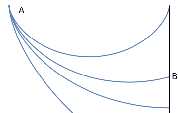
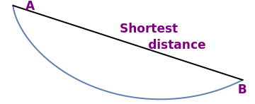
A famous problem of finding the planar curve on which a body subjected only to the force of gravity will slide (without friction) between two points in the least possible time was first posted by Galileo in 1638.
He proved that the time along two chords AC, CB, where C is any point of a circle including A and B, is less than the time along the single chord AB. As we increase the number of chords by choosing more points on the arc, time of travel becomes lesser and in the limit of the number of chords tending to infinity, the time becomes the least. He concluded that the quickest path along the arc of a circle with one of its ends being the endpoint of a vertical diameter of a circle. Galileo,
in his letter to his friend Guidobaldo del Monte on 29 November 1602, described the descent of heavy bodies along the arcs of circles and the chords subtended by them. Now we know that Galileo's conclusion about the curve being a circle is wrong.
Brachistochrone compared to other curves
However, in June 1696
the Swiss brilliant scientist
Johann Bernoulli (1667--1748) challenged mathematicians with the problem published in Acta Eruditorum. He called it the brachistochrone problem, which gave birth to the calculus of
variations. The word ``brachistochrone'' is derived
from two Greek words: brachistos
(βραχιστος), meaning
the ``shortest,'' and chronos (χρονος), meaning ``time.'' The problem he posed was the following:
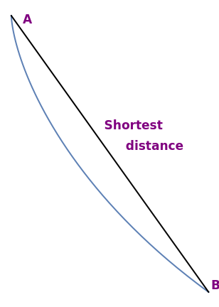
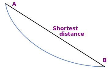
Given two points A and B in a vertical plane, with B below and to the right of A, what is the curve traced out by a point acted on only by constant gravity, which starts at A and reaches B in the shortest time.
Imagine a metal bead with a wire threaded through a hole in it, so that the bead can slide with no friction along the wire. How can one choose the shape of the wire so that the time of descent under gravity (from rest) is smallest possible? Upon choosing the Cartesian coordinates with downward y-axis and x-axis passes through the initial point, we are looking for a function y(x) such that y(0) = 0, and for which the time T of descent is minimized.
The steeper the curve, the faster it will move; however, it must convert some of this speed into motion in the x-direction to travel distance b because y(b) must be equal to B, the final destination.
The travel time along a path is given by the integral of the ratio of the arclength to the particle's speed. The movement of the bead is conservative, so we get
where m is the mass of the bead, v is its velocity, and g is the gravitational constant. Newton’s Law implies that for a mass m traveling on the arc s with angle θ from the downward direction
where for simplicity, we set the initial point at the origin: y0 = 0. Therefore, the above functional acts on the functions y ∈ C¹0,B([0,b]), the set of continuously differentiable functions vanishing at x = 0 and y(b) = B.
Observe that the Lagrangian density does not depend explicitly on the independent variable x. So we apply the Euler--Lagrange equation that gives a stationary curve. This curve, in general, not even provide a local maximum or minimum. So we get
\[
y' \,\frac{\partial L}{\partial y'} - L = c,
\]
where we have used the positive root. Although the brachistochrone equation
has a singular solution, it is
out of our interest because either the singular solution does not
satisfy the boundary condition or, when it does, the descent time
along it is not minimum.
The above equation is a separable one, so we have
This is a parametric representation of a curve called a cycloid, where r is the radius of the "wheel" that generates the cycloid and 0 ≤ θ ≤ Θ, provided that Θ is the unique solution of
One arch is produced by letting θ take on the values from 0 to 2π. The bottom point of this arch occurs when θ = π and has coordinates (rπ,2r). Thus, the slope m = B/b of the line from the cusp at the origin to the bottom point is 2r/rπ = 2/π.
One can show that there is a unique cycloid (the first half of the arch of the cycloid joining the origin with the point B is invertible) passing through any pair (0,0), (b,B) with 0 < B and that the unique cycloid is a global minimum for the functional T(y).
Johann Bernoulli gave a brilliant insight to the brachistochrone
problem by relating it to geometric optics, the branch of optics
that describes ray propagation. When a light beam (or ray) strikes a
smooth interface (a surface separating two transparent materials such
as air and glass or water and glass), the wave is in general partly
reflected and partly refracted (transmitted) into the second material,
as shown in the figure below. For simplicity we draw only one ray.
Fermat's Principle of Least Time:
light will follow the
path for which the time of travel is a minimum. The time T needed for
light to get point B from A is determined by
\[
T= \frac{\sqrt{a^2 + x^2}}{v_1} + \frac{\sqrt{b^2 + (c-x)^2}}{v_2} ,
\]
where v1 and v2 are the speeds of light in two different
materials. Since T is the minimum time to travel from A to B,
the derivative of T with respect to x must be zero, and we have
\[
\frac{x}{v_1 \sqrt{a^2 + x^2}} = \frac{c-x}{v_2 \sqrt{b^2 + (c-x)^2}}
\qquad\mbox{or}\qquad
\frac{\sin \alpha_1}{v_1} = \frac{\sin \alpha_2}{v_2} .
\]
This equation is called the law of refraction, or Snell's
law, after Dutch's astronomer and mathematician Willebrord
Snell (in Latin: Snellius) (1580 -- 1626).
where n is the coefficient describing the inhomogeneity of the medium. The corresponding Lagrangian is \( L = n\,\| {\bf x}'\| , \) where x = [x, y] in planar case. Let us introduce path-length as a new parameter
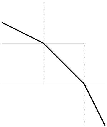
Let us consider the multilayer medium shown in Figure above. As the
incident ray passes from one material to another, it is always bent toward
or away from the normal according to Snell's law; namely,
\[
\frac{\sin \alpha_1}{v_1} = \frac{\sin \alpha_2}{v_2} = \frac{\sin
\alpha_3}{v_3} = \frac{\sin \alpha_4}{v_4} = \cdots .
\]
Johann Bernoulli recognized the similarity between the continuously increasing speed of light ray and the increasing speed of a heavy mass falling in a uniform gravitational field. Therefore, he argued that by following a law similar to that followed by a refracting light ray, the falling mass must take minimum time. He substitutes for the speed of light, v, in Snell’s law, the speed v acquired by a falling mass in a uniform gravitational field. The latter could easily be obtained by applying the law of conservation of energy that states that the sum of potential energy and kinetic energy of a falling mass must remain constant. In particular, if the falling mass starts from rest, then the sum must be zero for each point along the path. The proof is simple and elegant, combining fields of geometry and physics.
Suppose that the width of the layers approaches zero as a number of layers
increase to infinity. Then, as a limit, we have
\[
\frac{\sin \alpha}{v} = \mbox{constant}.
\]
Let us return to the brachistochrone problem and express v and α in terms of the height y and the slope y'. Suppose that a bead (like
a light ray) can choose the path to slide in a such a way that the time of
descent from the point A to the point B is a minimum. Therefore,
the above equation is valid.
The potential energy Π of a bead due to gravity is Π = mgy,
where y is the vertical coordinate of the bead. From the principle
of conservation of energy, it follows that
\[
mgy = \frac{m v^2}{2} \qquad \mbox{or} \qquad v= \sqrt{2 g y}.
\]
Note that the positive y-axis is increasing downward. On the other
hand,
\[
\sin\alpha = %\cos\beta = \frac{1}{\sec\beta} =
\frac{1}{\sqrt{1 + \tan^2 \beta}} = \frac{1}{\sqrt{1+ ( y' )^2}} ,
\]
where β = π/2 -α is the complementary angle to
α. Substitution of this expression for sinα and
\( v=\sqrt{2gy} \) into the equation \( \frac{\sin \alpha}{v} = \mbox{constant} \) yields
\[
y\left[ 1+ ( y' )^2 \right] = C ,
\]
where C is an arbitrary constant. This equation can
also be obtained by applying the Euler equation to the
total time T needed to slide down to the terminal position:
\[
T (y) = \int \frac{\mbox{distance}}{\mbox{rate}} = \int \frac{{\text d}s}{v} =
\int \frac{\sqrt{\dot{x}^2 + \dot{y}^2}}{\sqrt{2gy}}\,{\text d}t = \int_0^b
\frac{\sqrt{1+ y'^2}}{\sqrt{2gy}}\,{\text d}x \, ,
\]
where x = x(t), y = y(t) is the parametric equation of the slide
curve. Minimization of this functional T(y) leads us to
\( y\left[ 1+ ( y' )^2 \right] = C , \)
which upon differentiating gives another form of the
swiftest descent:
\[
y' \left[ 1 + ( y' )^2 + 2y y'' \right] =0 .
\]
Note that the general solution of the brachistochrone equation
contains two arbitrary constants that should be chosen to satisfy
the boundary conditions: the solution must go through the end points
A (which we choose as the origin for simplicity) and B. While the above equation has a singular solution, it is
out of our interest because either the singular solution does not
satisfy the boundary condition or, when it does, the descent time
along it is not minimum. From the brachistochrone equation, it follows that \( \displaystyle
y' = \frac{{\text d}y}{{\text d}x} = \left( \frac{C}{y} -1 \right)^{1/2} . \)
Separating variables leads to
\[
{\text d}x = \left( \frac{y}{C-y} \right)^{1/2} \,{\text d}y .
\]
We change the variable y by setting
\( \displaystyle \left[ \frac{y}{C-y} \right]^{1/2} = \tan\varphi . \)
Then since y = Csin² φ, we have
Integration yields
\[
x=\frac{C}{2}\,(2\varphi - \sin 2\varphi ) + C_1 ,
\]
where C1 is an arbitrary constant. We assume that the bead starts its
sliding from the origin, thus φ = 0 at x=0, y=0, and, hence, C1 = 0. As a result, we have
\[
x=\frac{C}{2}\,(2\varphi - \sin 2\varphi ) = C(\varphi - \sin
\varphi\, \cos\varphi ) , \qquad y= C\,\sin^2 \varphi =
\frac{C}{2} \,(1-\cos 2\varphi ) .
\]
Setting C/2 = r and 2φ = θ, we see that the curve that solves
the brachistochrone problem is just the cycloid. So this curve gives
a trade off between steepness versus path length.
■
Example:
The Friedmann equations are a set of equations in physical cosmology that govern the expansion of space in homogeneous and isotropic models of the universe within the context of general relativity. They were first derived by the Russian and Soviet physicist Alexander Friedmann (1888--1925) in 1922 from Einstein's field equations.
Let us begin with Newton’s mechanics, even though
the General Relativity Theory (GRT) must certainly be involved. However, as will
be seen, the GRT will come into play through a surprisingly simple artifice.
For the sake of simplicity, we consider a spherical universe. However, it should
be noted that the result holds in general.
Let r0 be the radius of the universe and ρ0 be the density of the masses at the present time t0. The radius as a function of time is
\[
r(t) = a(t) \cdot r_0 ,
\]
where the scale factor 𝑎 is dimensionless.
Assuming that the total mass of the universe is constant, we get
Substituting into \( r(t) = a(t) \cdot r_0 , \) we obtain \( \displaystyle \rho (t) = \rho_0 / a^3 (t) , \) Because of the homogeneity of the universe, we may assume that the total mass \( \displaystyle M = \rho_0 \cdot \frac{4\pi}{3} \,r_0^3 \) of the universe is concentrated at its center. Then by Newton’s law of motion, the gravitational force acting on point mass m at distance r from the center
of the universe is
\[
m \cdot \ddot{r} = - \frac{G m M}{r^2} = - \frac{G m}{r^2} \,\frac{4\pi}{3} \cdot r_0^3 \cdot \rho_0 .
\]
Using \( r(t) = a(t) \cdot r_0 , \) and dividing by m yields
We interpreter the integration constant as
K c², where c is the velocity of light and K is the curvature of the four-dimensional
space-time universe (dimension [K] = m-2).
■
Dumped harmonic oscillator
In many practical problems, a second order differential equation can be reduced to an exact equation.
For example, consider the equation of motion for the damped harmonic oscillator:
\[
\ddot{y} + 2\mu\,\dot{y} + \omega_0^2 y =0 ,
\]
be the roots of the characteristic equation \( \lambda^2 + 2\mu\, \lambda + \omega_0^2 =0 , \)
that is, \( \lambda_1 + \lambda_2 = 2\mu \) and
\( \lambda_1 \lambda_2 = \omega_0^2 . \) Multiplying both sides of the harmonic oscillator equation by
\( \mu (y,t) = e^{2\mu t} \left( \dot{y} + \mu y \right) , \) we obtain an exact equation:
Therefore, A is a constant of motion (which is also called the first integral of the equation). Note that
A is similar to the energy integral for a conservative system. The connection is easily seen if μ = 0,
corresponding to the undamped oscillator. Following Bohlin,
it can be shown that the second order differential equation for damped oscillator admits another first integral
\[
\frac{\left( \dot{y} + \lambda_1 y \right)^{\lambda_1}}{\left( \dot{y} + \lambda_2 y \right)^{\lambda_2}} =B >0
\]
or
\[
b = \ln B = \lambda_1 \ln\left( \dot{y} + \lambda_1 y \right) - \lambda_2 \ln \left( \dot{y} + \lambda_2 y \right) .
\]
Since this Hamiltonian depends explicitly on time, it does not represent a conserved quantity. This is just what we
should expect because we are dealing with a dissipative system.
Let us simplify the Hamiltonian with the transformation
This formula is rather remarkable because the new Hamiltonian does not depend explicitly on time, and so is
conservative. If we express the new Hamiltonian in old variables, we realize that the expression
Haws, L., Kiser, T., Exploring the brachistochrone problem, The American mathematical Monthly, 1995, Vol. 102, No. 4, pp. 328--336.
Johnson, N., The brachistochrone problem, The College Mathematics Journal, 2004, Vol. 35, No. 3, pp. 192--197.
Kimball, W.S., History of the Brachistochrone, Pi Mu Epsilon Journal, 1955, Vol. 2, No. 2, pp. 57--77.
Nahin, P.J., When Least is Best: How Mathematicians Discovered Many Clever Ways to Make Things as Small (or as Large) as Possible, Princeton, Princeton University Press, 2007.
Parsons, D.H., Exact Integration of the Space-Charge Equation for a Plane Diode: A Simplified Theory, Nature, 1963, Volume 200, October, pp. 126--127.
Zeng, J., A note on the brachistochrone problem, The College Mathematics Journal, 1996, Vol. 27, No. 3, pp. 206--208.
Return to Mathematica page
Return to the main page (APMA0330)
Return to the Part 1 (Plotting)
Return to the Part 2 (First Order ODEs)
Return to the Part 3 (Numerical Methods)
Return to the Part 4 (Second and Higher Order ODEs)
Return to the Part 5 (Series and Recurrences)
Return to the Part 6 (Laplace Transform)
Return to the Part 7 (Boundary Value Problems)