Return to computing page for the second course APMA0340
Return to Mathematica tutorial for the first course APMA0330
Return to Mathematica tutorial for the second course APMA0340
Return to the main page for the course APMA0330
Return to the main page for the course APMA0340
Return to Part III of the course APMA0330
Glossary
Error estimates
Now that we have learned how to use the numerical methods to find a numerical solution to simple first-order differential equations, we need to develop some practical guidelines to help us estimate the accuracy of various methods. Because we have replaced a differential equation by a difference equation, our numerical solution cannot be identically equal, in general, to the “true” solution of the original differential equation. In general, the discrepancy between the two solutions has two causes. One cause is that computers do not store numbers with infinite precision, but rather to a maximum number of digits that is hardware and software dependent. Most programming languages allow the programmer to distinguish between floating point or real numbers, that is, numbers with decimal points, and integer or fixed point numbers. Arithmetic with numbers represented by integers is exact. However in general, we cannot solve a differential equation using integer arithmetic. Hence, arithmetic operations such as addition and division, which involve real numbers, can introduce an error, called the roundoff error. For example, if a computer only stored real numbers to two significant figures, the product 2.1×3.2 would be stored as 6.7 rather than the exact value 6.72. The ignificance of roundoff errors is that they accumulate as the number of mathematical operations increases. Ideally we should choose algorithms that do not significantly magnify the roundoff error, for example, we should avoid subtracting numbers that are nearly the same in magnitude.
The other source of the discrepancy between the true answer and the computed answer is the error associated with the choice of algorithm. This error is called the truncation error. A truncation error would exist even on an idealized computer that stored floating point numbers with infinite precision and hence had no roundoff error. Because this error depends on the choice of algorithm and hence can be controlled by the programmer, you should be motivated to learn more about numerical analysis and the estimation of truncation errors. However, there is no general prescription for the best method for obtaining numerical solutions of differential equations. We will find in later sections that each method has advantages and disadvantages and the proper selection depends on the nature of the solution, which you might not know in advance, and on your objectives. How accurate must the answer be? Over how large an interval do you need the solution? What kind of computer are you using? How much computer time and personal time do you have?
In practice, we usually can determine the accuracy of our numerical solution by reducing the value of ∆t until the numerical solution is unchanged at the desired level of accuracy. Of course, we have to be careful not to choose ∆t too small, because too many steps would be required and the total computation time and roundoff error would increase.
In addition to accuracy, another important consideration is the stability of an algorithm. For example, it might happen that the numerical results are very good for short times, but diverge from the true solution for longer times. This divergence might occur if small errors in the algorithm are multiplied many times, causing the error to grow geometrically. Such an algorithm is said to be unstable for the particular problem. One way to determine the accuracy of a numerical solution is to repeat the calculation with a smaller step size and compare the results. If the two calculations agree to p decimal places, we can reasonably assume that the results are correct to p decimal places.
We present first the Mean Value Theorem from calculus that have an impact on numerical methods. A special case of this theorem was first described by Parameshvara (1370--1460), from the Kerala school of astronomy and mathematics in India. A restricted form of the theorem was proved by the French mathematician Michel Rolle (1652--1719) in 1691; the result was what is now known as Rolle's theorem, and was proved only for polynomials, without the techniques of calculus. The mean value theorem in its modern form was stated and proved by the French mathematician Baron Augustin-Louis Cauchy (1789--1857) in 1823.
Theorem (Mean Value Theorem): Let \( f:\, [a,b] \,\mapsto \,\mathbb{R} \) be a continuous function on the closed interval [𝑎,,b], and differentiable on the open interval (𝑎,b), where 𝑎<b. Then there exists some ξ in (𝑎,b) such that
Theorem (Cauchy Mean Value Theorem): If functions f and g are both continuous on the closed interval [a,b], and differentiable on the open interval (𝑎,b), then there exists some \( \xi \in (a,b) , \) such that
Theorem (Mean Value Theorem for definite integrals): If \( f:\, [a,b] \,\mapsto \,\mathbb{R} \) is integrable and \( g:\, [a,b] \,\mapsto \,\mathbb{R} \) is an integrable function that does not change sign on [a, b], then there exists some \( \xi \in (a,b) , \) such that
Error Estimates
We discussed so far different numerical algorithms to solve the initial value problems for first order differential equations:
The methods we introduce for approximating the solution of an initial value problem are called difference methods or discrete variable methods. The solution is approximated at a set of discrete points called a grid (or mesh) of points. An elementary single-step method has the form \( y_{n=1} = y_n + h\, \Phi (x_n, y_n ) \) for some function Φ called an increment function.
The errors incurred in a single integration step are
of two types:
1. The local truncation error or discretization
error - the error introduced by the approximation of the
differential equation by a difference equation.
2. Errors due to the deviation of the numerical solution
from the exact theoretical solution of the difference
equation. Included in this class are round-off errors, due
to the inability of evaluating real numbers with infinite
precision with the use of computer (i.e., computers usually
operate on fixed word length) , and errors which are incurred
if the difference equation is implicit and is not solved
exactly at each step.
If a multistep method is used, an additional source of
error results from the use of an auxiliary method (usually
a single-step method, e.g., Runge--Kutta method), to develop
the needed starting values for the multistep method.
In the numerical solution of an ODE, a sequence of approximations yn to the actual solution \( y = \phi (x ) \) is generated. Roughly speaking, the stability of a numerical method refers to the behavior of the difference or error, \( y_n - \phi (x_n ) , \) as n becomes large. To make our exposition simple, we consider the propagation of error in a one-step method by studying the particular representative one-step method of Euler:
Subtracting the latter from the former yields
The global discretization error ek is defined by
The local discretization error εk+1 is defined by
Theorem (Precision of Euler's Method): Assume that \( y= \phi (x) \) is the solution to the initial value problem
Example: Consider the initial value problem for the linear differential equation
h=(xf-x0)/n;
Y=y0;
For[i=0,i<n,i++,
Y=Y+f[x0+i*h,Y]*h]; Y]
n is number of steps
x0 = initial condition for x
y0 = initial condition for y
xf = final value of x at which y is desired.
f = slope function for the differential equation dy/dx = f(x,y)
Do[
Nn[i]=2^i;
H[i]=(xf-x0)/Nn[i];
AV[i]=EulerMethod[2^i,x0,y0,xf,f];
Et[i]=EV-AV[i];
et[i]=Abs[(Et[i]/EV)]*100.0;
If[i>0,
Ea[i]=AV[i]-AV[i-1];
ea[i]=Abs[Ea[i]/AV[i]]*100.0;
sig[i]=Floor[(2-Log[10,ea[i]/0.5])];
If[sig[i]<0,sig[i]=0];
] ,{i,0,nth}];
AV = approximate value of the ODE solution using Euler's Method by calling the module EulerMethod
Et = true error
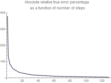
et = absolute relative true error percentage
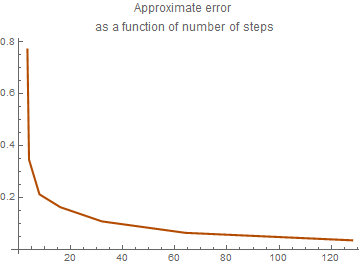
Ea = approximate error
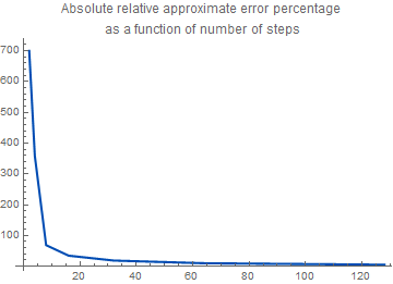
ea = absolute relative approximate error percentage
sig = least number of significant digits correct in approximation
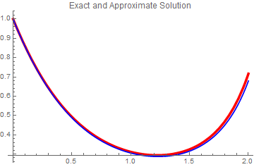
The following code uses Euler's Method to calculate intermediate step values for the purpose of displaying the solution over the range specified. The number of steps used is the maximum value, n (in this example, n=128).
X[0]=x0;
Y[0]=y0;
h=(xf-x0)/n;
For[i=1,i<=n,i++,
X[i]=x0+i*h;
Y[i]=Y[i-1]+f[X[i-1],Y[i-1]]*h; ];
plot2 = ListPlot[data, Joined -> True,
PlotStyle -> {Thickness[0.005], RGBColor[0, 0, 1]}];
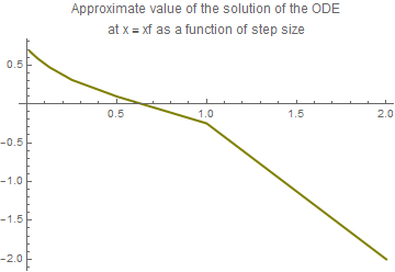
Now we compare the value at the final point (denoted by xf) with a step size
plot3 = ListPlot[data, Joined -> True,
PlotStyle -> {Thickness[0.006], RGBColor[0.5, 0.5, 0]}, PlotLabel ->
"Approximate value of the solution of the ODE\nat x = xf as a \ function of step size"]
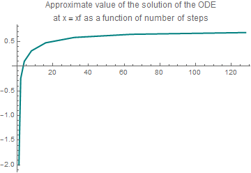
plot4 = ListPlot[data, Joined -> True,
PlotStyle -> {Thickness[0.006], RGBColor[0, 0.5, 0.5]}, PlotLabel -> "Approximate value of the solution of the ODE \n at x = xf as a \ function of number of steps "]
EV = (y /. First[soln])[xf]
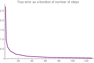
data = Table[{Nn[i], Et[i]}, {i, 0, nth}]; plot5 = ListPlot[data, Joined -> True,
PlotStyle -> {Thickness[0.006], RGBColor[0.5, 0, 0.5]}, PlotLabel ->
"True error as a function of number of steps"]
plot6 = ListPlot[data, AxesOrigin -> {0, 0},
Joined -> True, PlotStyle -> {Thickness[0.006], RGBColor[0.3, 0.3, 0.4]},
PlotLabel -> "Absolute relative true error percentage \n as a function of number of steps"]
plot7 = ListPlot[data, AxesOrigin -> {0, 0},
Joined -> True, PlotStyle -> {Thickness[0.006], RGBColor[0.7, 0.3, 0]},
PlotLabel -> "Approximate error \nas a function of number of steps"]
plot9 = ListPlot[data, AxesOrigin -> {0, 0},
Joined -> True, PlotStyle -> {Thickness[0.006], RGBColor[0, 0.3, 0.7]},
PlotLabel -> "Absolute relative approximate error percentage \nas a function of \ number of steps"]
Theorem (Precision of Heun's Method): Assume that \( y= \phi (x) \) is the solution to the initial value problem
Accuracy
Sometimes you may be interested to find out what methods are being used in NDSolve.
Here you can see the coefficients of the default 2(1) embedded pair.
{{{1}, {1/2, 1/2}}, {1/2, 1/2, 0}, {1, 1}, {-(1/2), 2/3, -(1/6)}}
You also may want to compare some of the different methods to see how they perform for a specific problem.
Implicit Runge--Kutta methods have a number of desirable properties.
The Gauss--Legendre methods, for example, are self-adjoint, meaning that they provide the same solution when integrating forward or backward in time.
http://reference.wolfram.com/language/tutorial/NDSolveImplicitRungeKutta.html
A generic framework for implicit Runge--Kutta methods has been implemented. The focus so far is on methods with interesting geometric properties and currently covers the following schemes:
"ImplicitRungeKuttaGaussCoefficients"
"ImplicitRungeKuttaLobattoIIIACoefficients"
"ImplicitRungeKuttaLobattoIIIBCoefficients"
"ImplicitRungeKuttaLobattoIIICCoefficients"
"ImplicitRungeKuttaRadauIACoefficients"
"ImplicitRungeKuttaRadauIIACoefficients"
The derivation of the method coefficients can be carried out to arbitrary order and arbitrary precision.
Errors in Numerical Approximations
The main question of any approximation is whether the numerical approximations \( y_1 , y_2 , y_3 , \ldots \) approach the corresponding values of the actual solution? We want to use a step size that is small enough to ensure the required accuracy. An unnecessarily small step length slows down the calculations and in some cases may even cause a loss of accuracy.
There are three fundamental sources of error in approximating the solution of an initial value problem numerically.
- The formula, or algorithm, used in the calculations is an approximating one.
- Except for the first step, the input data used in the calculations are only approximations to the actual values of the solution at the specified points.
- The computer used for the calculations has finite precision; in other words, at each stage only a finite number of digits can be retained.
Let us temporarily assume that our computer can execute all computations exactly; that is, it can retain infinitely many digits (if necessary) at each step. Then the difference En between the actual solution \( y = \phi (x) \) of the initial value problem \( y' = f(x,y), \quad y(x_0 ) = y_0 \) and its numerical approximation yn at the point x = xn is given by
However, in reality we must carry out the calculations using finite precision arithmetic because of the limited accuracy of any computing equipment. This means that we can keep only a finite number of digits at each step. This leads to a round-off error Rn defined by
Therefore, the total error is bounded by the sum of the absolute values of the global truncation and round-off errors. The round-off error is very difficult to analyze and it is beyond of the scope of our topic. To estimate the global error, we need one more definition.
As we carry the solution over many steps we would expect the values yn and \( \phi (x_n ) \) to diverge further and further apart. The local truncation error is concerned only with the direvgence produced within the present step so that it is appropriate to reinitialize yn to the value of \( \phi (x_{n} ) \) in studying this source of error. The corresponding solution to the initial value problem
Roundoff Errors
Rounding errors are not random and are typically correlated. When rounding error leads to trouble, instead of thinking about a mysterious rounding-error accumulation, you should analyze operations that may cause this error.
IV. Regular Plotting vs Log-Plotting
Plotting the absolute value of the errors for Taylor approximations, such as the ones from the previous example, is fairly easy to do in normal plotting.
The normal plotting procedure involves taking all of the information regarding the Taylor approximations and putting them into one file, then calculate the exact solution, then find the difference between each approximation and the exact solution, and plotting the solution.
Looking at the code, the syntax is pretty much self-explanatory. The only part that may confuse students is the syntax for the plot command. The plot command need not be in the same syntax as the file has it. If you wish to, you can alter the syntax to form a curve instead of dots.
Log-plotting is not much different than plotting normally. In other programs such as Mathematica, there are a couple of fixes to make, but in Maple only one line of code is required, as seen in the file. Make sure that before you use the logplot command to open the plots package.
Now, let’s compare the exact value and the values determined by the polynomial approximations and the Runge-Kutta method.
| x values | Exact | First Order Polynomial | Second Order Polynomial | Third Order Polynomial | Runge-Kutta Method |
| 0.1 | 1.049370088 | 1.050000000 | 1.049375000 | 1.049369792 | 1.049370096 |
| 0.2 | 1.097463112 | 1.098780488 | 1.097472078 | 1.097462488 | 1.097463129 |
| 0.3 | 1.144258727 | 1.146316720 | 1.144270767 | 1.144257750 | 1.144258752 |
| 0.4 | 1.189743990 | 1.192590526 | 1.189758039 | 1.189742647 | 1.189744023 |
| 0.5 | 1.233913263 | 1.237590400 | 1.233928208 | 1.233911548 | 1.233913304 |
| 0.6 | 1.276767932 | 1.281311430 | 1.276782652 | 1.276765849 | 1.276767980 |
| 0.7 | 1.318315972 | 1.323755068 | 1.318329371 | 1.318313532 | 1.318316028 |
| 0.8 | 1.358571394 | 1.364928769 | 1.358582430 | 1.358568614 | 1.358571457 |
| 0.9 | 1.397553600 | 1.404845524 | 1.397561307 | 1.397550500 | 1.397553670 |
| 1.0 | 1.435286691 | 1.443523310 | 1.435290196 | 1.435283295 | 1.435286767 |
| Accuracy | N/A | 99.4261% | 99.99975% | 99.99976% | 99.99999% |
You will notice that compared to the Euler methods, these methods of approximation are much more accurate because they contains much more iterations of calculations than the Euler methods, which increases the accuracy of the resulting y-value for each of the above methods.
- Gezerlis, A, Williams, M., Six-textbook mistakes in computational physics, American Journal of Physics, 2021, Vol. 89, No. 1, pp. 51--60.
- Higham, N.J., Accuracy and Stability of Numerical Algorithms, 2002, 2nd edition, SIAM (Society for Industrial and Applied Mathematics), Pennsylvania.
Return to Mathematica page
Return to the main page (APMA0330)
Return to the Part 1 (Plotting)
Return to the Part 2 (First Order ODEs)
Return to the Part 3 (Numerical Methods)
Return to the Part 4 (Second and Higher Order ODEs)
Return to the Part 5 (Series and Recurrences)
Return to the Part 6 (Laplace Transform)
Return to the Part 7 (Boundary Value Problems)