Preface


Taylor's power series method is the main topic of this section.

Return to computing page for the first course APMA0330
Return to computing page for the second course APMA0340
Return to Mathematica tutorial for the first course APMA0330
Return to Mathematica tutorial for the second course APMA0340
Return to the main page for the course APMA0330
Return to the main page for the course APMA0340
Return to Part V of the course APMA0330

Our main method to solve nonlinear and variable coefficient linear differential equations is expansion of solutions into power series. Before the middle of 20th century, it was the standard method for attacking problems of this kind and many of the famous equations such as Legendre and Chebyshev equations have series solutions named after them. With the availability of computers, the power series came to prominence once again. In this tutorial, we present four algorithms for solving nonlinear differential equations with power series:

Taylor Series Method


When solving initial value problems (IVPs) for ordinary differential equations (ODEs) using power series method, we always assume that the solution y(x) exists and smooth enough to be approximated by Taylor's polynomial of N-th degree
\begin{equation} \label{EqTaylor.1} T_N (x) = c_0 + c_1 \left( x - x_0 \right) + c_2 \left( x - x_0 \right)^2 + \cdots + c_N \left( x - x_0 \right)^N = \sum_{k=0}^N c_k \left( x - x_0 \right)^k , \end{equation}
where coefficients are
\begin{equation} \label{EqTaylor.2} c_n = c_n (y) = \frac{1}{n!}\,y^{(n)} \left( x_0 \right) = \frac{1}{n!}\,\lim_{x\to x_0} \texttt{D}^n y(x) , \qquad \texttt{D} = \frac{{\text d}^n}{{\text d} x^n} . \end{equation}
If solution y(x) is a holomorphic function, then the error of approximation by Taylor's polynomial approaches zero when N → ∞. For first order differential equations (written in normal form):
\begin{equation} \label{EqTaylor.3} \frac{{\text d}y}{{\text d} x} = f \left( x , y \right) , \qquad y \left( x_0 \right) = y_0 , \end{equation}
the coefficients in Eq.\eqref{EqTaylor.2} are determined by differentiation of the slope function:
\begin{equation} \label{EqTaylor.4} c_n = c_n (y) = \frac{1}{n!}\,y^{(n)} \left( x_0 \right) = \frac{1}{n!}\,\lim_{x\to x_0} \, \frac{\partial^{n-1} f(x,y(x))}{\partial x^{n-1}} , \qquad n = 1, 2, \ldots . \end{equation}
This leads to application of the famous Faà di Bruno's Formula that gives an explicit expression for the n-th derivative of the composition of two functions. However, the number of terms in this formula grows exponentially, according to the asymptotic partition formula by J. V. Uspensky (1920). So there is no chance to obtain explicit expressions for all Taylor's coefficients, in general. If a slope function is a polynomials, then all Taylor's coefficients will eventually contain only finite number of terms.

Differentiating Eq.\eqref{EqTaylor.3} with respect to x, we get

\[ y'' = f_x + f\,f_y . \]
Similarly
\[ y''' = f_{xx} + f^2 f_{yy} + 2\,f\,f_{xy} + f_x f_y + f\,f_y^2 , \]
where fx, fx, … represent the partial derivatives of f with respect to x and y and so on. The values of \( \displaystyle y'_0 = y' \left( x_0 \right) , \ y''_0 = y'' \left( x_0 \right) , \ldots \) can be obtained by putting x = x0 and y = y0. If y(x) is the exact solution, then the Taylor’s series for y(x) around x = x0 is given by
\begin{equation} \label{EqTaylor.5} y(x) = y_0 + y'_0 \left( x - x_0 \right) + \frac{y''_0}{2!} \left( x - x_0 \right)^2 + \frac{y'''_0}{3!} \left( x - x_0 \right)^3 + \cdots , \end{equation}
which gives the value of y for every value of x for which Eq.\eqref{EqTaylor.5} converges.


First order separable equations


Although the initial value problem for a separable differential equation can be solved by separation of variables, we demonstrate the Taylor's series approach on this particular class of equations. Let us consider the initial value problem (IVP for short) for a separable equation
\[ y' \left( x \right) = f \left( x \right) \,g \left( y \right) , \qquad y \left( x_0 \right) = y_0 . \]
The first derivative at the initial point follows immediately from the given differential equation
\[ y' \left( x_0 \right) = f \left( x_0 \right) \,g \left( y_0 \right) . \]
Next differentiation yields
\[ y''(x) = f' (x)\, g (y) + f(x)\, g' (x)\, y' = f' (x)\, g (y) + f(x)\, g' (x)\, f(x)\, g(y) = f' (x)\, g (y) + f^2 (x)\, g' (y)\, \, g(y) , \]
where we used the given differential equation to determine the first derivative of y'(x). We check the answer with Mathematica
der[x_] = f[x]*Composition[g, y][x];
D[der[x], x] /. y'[x] -> der[x]
g[y[x]] Derivative[1][f][x] + f[x]^2 g[y[x]] Derivative[1][g][y[x]]
Then the value of the second coefficient in the Taylor's series becomes
\[ y'' \left( x_0 \right) = f' \left( x_0 \right) g \left( y_0 \right) + f^2 \left( x_0 \right) g' \left( y_0 \right) g\left( y_0 \right) . \]
To find the third coefficient, we have to differentiate the expression for the second derivative:
\[ y''' (x) = \frac{\text d}{{\text d}x} \, y'' = \frac{\text d}{{\text d}x} \left[ f' (x)\,g(y) + f^2 (x)\, g' (y)\, \, g(y) \right] = f''\,g + 3\,f\,f'\,g\,g' + f^2 \left[ g''\,g^2 + \left( g' \right)^2 g \right] . \]
We check with Mathematica:
der[x_] = f[x]*Composition[g, y][x];
y2[x_] = D[der[x], x] /. y'[x] -> der[x];
der2[x_] = D[y2[x], x] /. y'[x] -> der[x]
3 f[x] g[y[x]] Derivative[1][f][x] Derivative[1][g][y[x]] + f[x]^3 g[y[x]] Derivative[1][g][y[x]]^2 + g[y[x]] (f^\[Prime]\[Prime])[x] + f[x]^3 g[y[x]]^2 (g^\[Prime]\[Prime])[y[x]]
Although it is clear how to find the next derivative, the number of terms for its evaluation grows as a snow ball.

Example: Consider the differential equation

\[ y' = f(x)\, y^m , \]
where m is a real number. Using the slope function f(x) ym, we obtain from Eq.\eqref{EqTaylor.3} that
\[ y'' = f' (x)\, y^m + m\,f(x)\, y^{m-1} f(x)\, y^m = f' (x)\, y^m + m\,f^2 (x)\, y^{2m-1} , \]
Its next derivatives are
\begin{align*} y''' &= f'' (x)\, y^m + 3m\,f' (x)\,f (x)\, y^{2m-1} + m \left( 2m-1 \right) y^{3m-2} t'^3 (x)\,f(x) , \\ y^{(4)} &= \end{align*}
For particular values of m this sequence may terminante at a finite value of n. If m ≠ 1, the general solution is
\[ \sum_{n\ge 0} \frac{(-1)^n}{n!}\, \left( 1- m \right)^n \binom{1/(1-m)}{n} \,h^n (x) y^{mn-n+1} = C. \]

Consider a particular separable equation

\[ y' = f(x) \, y^{1/2} \qqiad \frac{{\text d} y}{\sqrt{y}} = f(x)\,{\text d} x . \]
Integration gives the general solution in implicit form:
\[ 2\,y^{1/2} = \int_{x_0}^x f(s)\,{\text d}s + C . \]
The g-functions from Eq.\eqref{EqIter.1} are
\[ g_1 (y) = y^{1/2} , \qquad g_2 (y) = \frac{1}{2} , \qquad g_n = 0, \quad n=3,4,\ldots . \]
The series solution is reduced to
\[ y - h(x)\, y^{1/2} + \frac{1}{4}\, h(x)^2 = C \qquad \Longrightarrow \qquad y = \left[ \frac{1}{2}\,h(x) + C \right]^2 . \]
   ■


Generalized Riccati equation


Consider the differential equation
\begin{equation} y' = f(x) + g(y) \qquad\mbox{with} \qquad h' (x) = f(x) \quad\mbox{and} \quad y(x_0 ) = y_0 . \label{EqIter.3} \end{equation}
Differentiating both sides, we get
\[ y'' (x) = f' (x) + g' (y) \left[ f(x) + g(y) \right] . \]
Next derivative will be
\[ y''' = f'' (x) + f'(x)\,g'(y(x)) + \left( f(x) + g(y) \right) g' (y) + \left( f(x) + g(y) \right)^2 g'' (y) . \]
We check with Mathematica:
der[x_] = f[x]+Composition[g, y][x];
y2[x_] = D[der[x], x] /. y'[x] -> der[x];
der2[x_] = D[y2[x], x] /. y'[x] -> der[x]
Derivative[1][g][ y[x]] (Derivative[1][f][ x] + (f[x] + g[y[x]]) Derivative[1][g][y[x]]) + ( f^\[Prime]\[Prime])[ x] + (f[x] + g[y[x]])^2 (g^\[Prime]\[Prime])[y[x]]
In general, we get
\[ \frac{{\text d}^{n+1} y}{{\text d} x^{n+1}} = \frac{{\text d}^{n} f(x)}{{\text d} x^{n}} + \frac{\partial^n}{\partial x^n} \,g(y(x)) , \]
which requires application of Faà di Bruno's formula for generalized chain rule.

Example: Consider the Riccati equation

\[ y' = y^2 + 2x , \qquad y(0) = a. \]
Integrating both sides, we obtain
\[ y - a = x^2 + \int_0^x y^2 (s)\,{\text d} s = x^2 + \left[ s\,y^2 (s) \right]_{s=0}^{s=x} - \int_0^x s\,2y(s)\left( 2s + y^2 (s) \right) {\text d} s . \]
We simplify the result as
\[ y - a = x^2 + x\,y^2 - 4 \int_0^x s^2 y(s)\, {\text d} s - 2 \int_0^x \frac{\text d}{{\text d} s} \left( \frac{s^2}{2} \right) y^3 (s) \, {\text d} s . \]
Next integration by parts yields
\begin{align*} \int_0^x s^2 y(s)\, {\text d} s &= \left[ \frac{s^3}{3}\, y(s) \right]_{s=0}^{s=x} - \int_0^x \frac{s^3}{3} \left( y^2 (s) + 2s \right) {\text d} s \\ &= \frac{x^3}{3}\, y - \int_0^x \frac{\text d}{{\text d} s} \left( \frac{s^4}{4\cdot 3} \right) y^2 (s) \, {\text d} s - \frac{2}{15}\, x^5 , \\ \int_0^x \frac{\text d}{{\text d} s} \left( \frac{s^2}{2} \right) y^3 (s) \, {\text d} s &= \left[ \frac{s^2}{2}\, y^3 \right]_{s=0}^{s=x} - \int_0^x \frac{s^2}{2}\,3\,y^2 (s) \left( y^2 (s) + 2s \right) {\text d} s \\ &= \frac{x^2}{2}\,y^3 - \int_0^x y^4 (s) \,\frac{\text d}{{\text d} s} \left( \frac{s^3}{2} \right) {\text d} s - \int_0^x 3\,s^3 y^2 (s) \, {\text d} s . \end{align*}
Disregarding integral terms, we obtain a polynomial approximation
\[ y - a = x^2 + x\,y^2 - \frac{4}{3}\,x^3 y + \frac{8}{15}\, x^5 - x^2 y^3 . \]
      We plot the implicit approximation along with the true solution:
contour2 = ContourPlot[ y - 1 == x^2 + x*y^2 - (4/3)*x^3 *y + (8/15)*x^5 - x^2 y^3, {x, 0, 0.8}, {y, 0.8, 1.6}, ContourStyle -> ColorData[10] /@ Range[10], BaseStyle -> Thickness[0.007]];
s = NDSolve[{y'[x] == y[x]^2 + 2*x, y[0] == 1}, y, {x, 0, 0.8}];
sol = Plot[Evaluate[y[x] /. s], {x, 0, 0.8}, PlotStyle -> {Orange, Thickness[0.01]}, PlotRange -> {0.8, 1.6}];
t1 = Graphics[ Text[Style["True solution", Orange, FontSize -> 18], {0.46, 1.5}]];
t2 = Graphics[ Text[Style["Approximation", Purple, FontSize -> 18], {0.5, 1.15}]];;
Show[contour2, sol, t1, t2]
       True solution (in orange) and its approximation.            Mathematica code

   ■


Second order linear differential equations


For a given second order differential equation
\begin{equation} \label{EqTaylor.6} y'' + p(x)\,y' + q(x)\,y = f(x), \qquad y\left( x_0 \right) = y_0 , \quad y'\left( x_0 \right) = y_1 , \end{equation}
the coefficients p and q are assumed to be a holomorphic functions. From Eq.\eqref{EqTaylor.6}, the second Taylor's coefficient follows immediately
\[ c_2 = \frac{1}{2}\, y'' \left( x_0 \right) = -\frac{1}{2}\, p \left( x_0 \right) y_1 - \frac{1}{2}\, q\left( x_0 \right) y_0 + \frac{1}{2}\, f\left( x_0 \right) . \]
All next dedrivatives are obtained upon differentiation both sides of the equation:
\[ y'' = f(x) - p(x)\, y' - q(x)\, y(x) . \]
Let us illustrate the Taylor series method with a typical linear differential equation subject to some initial conditions
\[ y'' (t) - 2t\,y' (t) + 3\,y(x) = \sin t , \qquad y(0) =1, \quad y' (0) = 0. \]
We assume an ansatz that the solution is a holomorphic function
\[ y(t) = 1 + \sum_{n\ge 1} c_n t^n . \]
First, we define this problem in Mathematica notebook:
ode = y''[t] - 2*t*y'[t] + y[t] - Sin[t] == 0;
ics = {y'[0] == 0, y[0] == 1};
Then we create a differentail operator to generate this ode
odeOperator = D[#, {t, 2}] - 2*t*D[#, t] + 3*# - Sin[t] &;
Now set up our Taylor's series as a symbolic expansion using derivatives of `y` evaluated at the origin. I use an order of 15 but that is something one would probably make as an argument to a function, if automating all this.
xx = Series[y[t], {t, 0, 15}];
Next apply the differential operator and add the initial conditions. Then find a solution that makes all powers of `t vanish.
soln = SolveAlways[Join[{odeOperator[xx] == 0}, ics], t];
Let's look at the Taylor's polynomial.
truncatedSol = Normal[xx /. soln[[1]]]
1 - (3 t^2)/2 + t^3/6 - t^4/8 + t^5/60 - t^6/48 + t^7/336 - ( 3 t^8)/896 + (41 t^9)/90720 - (13 t^10)/26880 + ( 2461 t^11)/39916800 - (221 t^12)/3548160 + (7793 t^13)/1037836800 - ( 17 t^14)/2365440 + (215087 t^15)/261534873600
\[ y(t) = 1 - \frac{3 t^2}{2} + \frac{t^3}{6} - \frac{t^4}{8} + \frac{t^5}{60} - \frac{t^6}{48} + \frac{t^7}{336} - \frac{3\,t^8}{896} + \frac{41\,t^9}{90 720} - \frac{13\,t^{10}}{26 880} + \cdots . \]
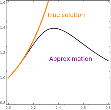
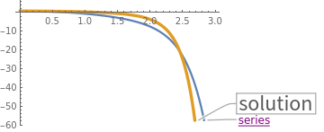
To assess how accurate it might be we compare Taylor's polynomail of degree 15 with "true" solution calculated by Mathematica standard command NDSolve:
approxSol = NDSolve[Join[{ode}, ics], y[t], {t, 0, 3}];
      We plot the 15th degree polynomail approximation along with the true solution:
Plot[{Callout[truncatedSol, "series", Automatic, LabelStyle -> Directive[Medium, Purple, Underlined]], Callout[y[t] /. approxSol[[1]], "solution", Automatic, Frame -> True, LabelStyle -> "Subtitle"]}, {t, 0, 3}, PlotStyle -> {{Thickness[0.01]}, {Thickness[0.015]}}]
       True solution and its series approximation.            Mathematica code

Since Mathematica knows how to find a Taylor's series approximation, you also have to understand the technique. Expressing the second (highest) derivative from the equation, we obtain
\[ y'' = 2t\, y' - 3\, y(t) + \sin t. \]
Taking the limit as t → 0, we get the value of the first coefficient in its Maclaurin series:
\[ y''(0) = - 3\, y(0) + \sin 0 = -3 \qquad \Longrightarrow \qquad c_2 = \frac{1}{2}\, y'' (0) = -\frac{3}{2} . \]
Then we differentiate the expression for the second derivative and take the limit as t → 0. This gives
\begin{align*} y^{(3)} &= \frac{\text d}{{\text d}t} \left( 2t\, y' - 3\, y(t) + \sin t \right) = 2t\, y'' - y' + \cos t \qquad \Longrightarrow \qquad c_3 = \frac{1}{3!} \,y^{(3)} (0) = \frac{1}{6} , \\ y^{(4)} &= \frac{\text d}{{\text d}t} \, y^{(3)} (t) = 2t\, y^{(3)} + y'' - \sin t \qquad \Longrightarrow \qquad c_4 = \frac{1}{4!} \,y^{(4)} (0) = -\frac{3}{4!} = -\frac{1}{8} , \\ y^{(5)} &= \frac{\text d}{{\text d}t} \, y^{(4)} (t) = 2t\, y^{(4)} + 3\, y^{(3)} - \cos t \qquad \Longrightarrow \qquad c_5 = \frac{1}{5!} \,y^{(5)} (0) = \frac{2}{5!} = \frac{1}{60} , \end{align*}
and so on. So if you know calculus and patient enough, you can determine as many coefficients as you wish. This is because the given differential equation has polynomail coefficients of degree at most 1. For example,
\[ y^{(6)} (t) = 2t\,y^{(5)} (t) + 5\, y^{(4)} (t) - \sin t \qquad \Longrightarrow \qquad c_6 = \frac{1}{6!} \,y^{(6)} (0) = \frac{1}{6!} \, (-15) = -\frac{1}{48} . \]


Second order nonlinear differential equations


Example: Consider the Abel equation, named after Niels Henrik Abel

\[ y' = y^3 + x \]
   ■


  1. Shih-Hsiang Chang and I-Ling Chang, A new algorithm for calculating one-dimensional differential transform of nonlinear functions, Applied Mathematics and Computation 2008, Vol. 195, Issue 2, pp. 799–808; doi: 10.1016/j.amc.2007.05.026
  2. Fairen, V., Lopez, V., Conde, L., Power series approximation to solutions of nonlinear systems of differential equations, American Journal of Physics, 1988, Vol. 56, Issue , pp. 57--61; https://doi.org/10.1119/1.15432
  3. Uspensky, J.V., Asymptotic formulae for numerical functions which occur in the theory of partitions (in Russian), Izv. Akad. Nauk SSSR, 1920, 14 pp. 199—218.


Return to Mathematica page
Return to the main page (APMA0330)
Return to the Part 1 (Plotting)
Return to the Part 2 (First Order ODEs)
Return to the Part 3 (Numerical Methods)
Return to the Part 4 (Second and Higher Order ODEs)
Return to the Part 5 (Series and Recurrences)
Return to the Part 6 (Laplace Transform)
Return to the Part 7 (Boundary Value Problems)