Preface


This section presents important applications to geometry; namely, it discusses deriving orthogonal trajectories based on differential equations.

Return to computing page for the first course APMA0330
Return to computing page for the second course APMA0340
Return to Mathematica tutorial for the second course APMA0340
Return to the main page for the course APMA0330
Return to the main page for the course APMA0340
Return to Part II of the course APMA0330

Orthogonal Trajectories


Two lines \( \ell_1 \quad\mbox{and}\quad \ell_2 , \) with slopes m1 and m2, respectively, are orthogonal or perpendicular if their slopes satisfy the relationship \( m_1 m_2 =-1 . \) Two curves are orthogonal or perpendicular at a point if their respective tangent lines to the curves at that point are perpendicular.

The word orthogonal comes from the Greek ορθη (right) and γωνια (angle); the word trajectory comes from the Latin trajectus (cut across). Therefore, a curve that cuts across certain others at right angles is called an orthogonal trajectory of those others.

Now we extend this definition to the family of curves that form the general solution of the differential equation. Suppose that the differential equation \( y' = f(x,y) \) has the family of solutions in implicit form \( F(x,y) = C , \) where C is an arbitrary constant. We refer to the set of curves on the plane as the family of orthogonal trajectories is they form the general solution to the differential equation \( y' = - 1/f(x,y) . \) For example, a family of exponential curves bx and b-x/(lnb)² are orthogonal.

Manipulate[ Plot[Evaluate@ Table[Tooltip[{b^x + a/3, 1/2^x/(Log[b])^2 + a/2}, a], {a, 1, 5}], {x, -0.1, 1.5}, AspectRatio -> Automatic], {b, 2, 5, Appearance -> "Labeled"}]
or
Plot[Evaluate@ Table[Tooltip[{2^x + a/3, 1/2^x/(Log[2])^2 + a/2}, a], {a, 1, 5}], {x, -0.1, 1.5}, AspectRatio -> Automatic]
Hence, two families of solutions are orthogonal if they are solutions of the differential equations:
\[ \frac{{\text d}y}{{\text d}x} = f(x,y) \qquad\mbox{and}\qquad \frac{{\text d}y}{{\text d}x} = \frac{-1}{f(x,y)} \]
or
\[ M(x,y)\,{\text d}x + N(x,y)\,{\text d}y =0 \qquad\mbox{and}\qquad N(x,y)\,{\text d}x - M(x,y)\,{\text d}y =0 . \]

Example: : 
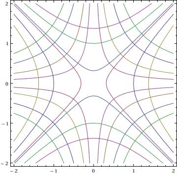
Suppose that we are given the family of curves x*y=c, where c is a constant. These are hyperbolas in quadrants 1 and 3 for c>0 or quadrants 2 and 4 for c<0, having the axes as asymptotes. They are rectangular hyperbolas because their asymptotes are perpendicular. The differential equation of the family is

\[ x y' + y =0, \qquad\mbox{or}\qquad \frac{{\text d}y}{{\text d}x} = - \frac{y}{x} . \]
The orthogonality condition says that the equation of the orthogonal curves should be \( -{\text d}x/{\text d}y = -y/x \) or \( -{\text d}y/{\text d}x = y/x . \) The latter has the general solution (after separation of variables): \(y^2 = x^2 +c. \) Now we plot these curves.
a := ContourPlot[{x y == 1, x y == 0.2, x y == 0.5, x y == 1.5,
x y == -1, x y == -0.2, x y == -0.5, x y == -1.5}, {x, -2, 2}, {y, -2, 2}]
b := ContourPlot[{x^2 == y^2 + 1, x^2 == y^2 + 0.1, x^2 == y^2 + 1.9,
x^2 == y^2 - 1, x^2 == y^2 - 0.1, x^2 == y^2 - 1.9}, {x, -2, 2}, {y, -2, 2}]
Show[a, b]

Example: : 
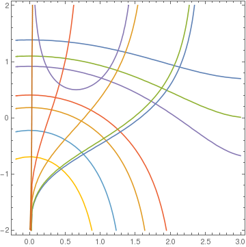
The separable differential equation \( e^y \,{\text d}y = \sin x\,{\text d}x \) defines its family of solutions: \( e^y = \cos x + c . \) The orthogonal trajectories to it are obtained by solving the differential equation

\[ \sin x\,{\text d}y + e^y \,{\text d}x =0 \qquad \Longrightarrow \qquad e^{-y} \,{\text d}y = \frac{{\text d}x}{\sin x} . \]
Integration yields the general solution \( \ln \left\vert \tan \frac{x}{2} \right\vert + e^{-y} = c , \) which is a family (depending on parameter c) of orthogonal trajectories to the general solution of \( e^y \,{\text d}y = \sin x\,{\text d}x . \)
a := ContourPlot[{Exp[y] - Cos[x] == 3, Exp[y] - Cos[x] == 0.2,
Exp[y] - Cos[x] == 2, Exp[y] - Cos[x] == 0.5,
Exp[y] - Cos[x] == 1.5, Exp[y] - Cos[x] == -2,
Exp[y] - Cos[x] == -0.2, -Cos[x] + Exp[y] == -0.5, -Cos[x] +
Exp[y] == -1.5}, {x, -0.2, 3}, {y, -2, 2}]
b := ContourPlot[{Log[Tan[x/2]] == -Exp[-y] + 1,
Log[Tan[x/2]] == -Exp[-y] + 0.1, Log[Tan[x/2]] == -Exp[-y] + 0.9,
Log[Tan[x/2]] == -Exp[-y] - 1, x Log[Tan[x/2]] == -Exp[-y] - 0.1,
Log[Tan[x/2]] == -Exp[-y] - 3.9}, {x, -0.2, 3}, {y, -2, 2}]
Show[a, b]
   ■


Orthogonal trajectories: polar coordinates


Consider a curve whose equation is expressed in polar coordinates (r,θ). In calculus it is shown that the angle ψ, measured positive in the counterclockwise direction from the radius vector to the tangent line at a point, is given by
\[ \tan\psi = r\,\frac{{\text d}\theta}{{\text d}r} . \]
If two curves are orthogonal at some point having angles ψ1 and ψ2, then ψ2 = ψ1 + π/2. So \( \tan\psi_2 = - \cot\psi_1 = -1/\tan\psi_1 . \) Hence, if two curves are to cut one another at right angles, then at the point of intersection the value of the product \( \displaystyle r\,\frac{{\text d}\theta}{{\text d}r} \) for one curve must be the negative reciprocal of the value of that product for the other curve.

When polar coordinates are used, suppose a family of curves forms the general solution to the differential equation \( P(r,\theta )\,{\text d}r + Q(r,\theta )\,{\text d}\theta = 0 . \) Then \( \displaystyle r\,\frac{{\text d}\theta}{{\text d}r} = - \frac{r\,P}{Q} . \) Hence, the family of the orthogonal trajectories of the solutions must be solutions of the equations

\[ \frac{{\text d}\theta}{{\text d}r} = f(r,\theta ) \qquad\mbox{and}\qquad \frac{{\text d}\theta}{{\text d}r} = \frac{-1}{r^2 f(r,\theta )} \]
or
\[ P(r,\theta )\,{\text d}r + Q(r,\theta )\,{\text d}\theta =0 \qquad\mbox{and}\qquad Q(r,\theta )\,{\text d}r - r^2 P(r,\theta )\,{\text d}\theta =0 . \]

Example: 
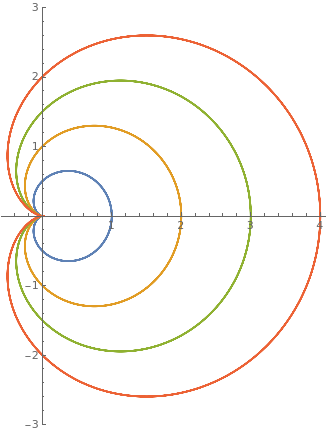
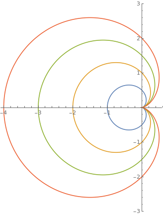
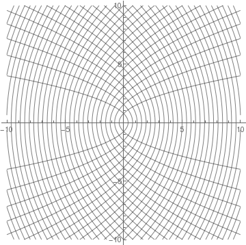
Let us find the orthogonal trajectories of the family of cardioids \( r = a \left( 1 + \cos\theta \right) . \) We plot a few curves with Mathematica

parameters = {0.5, 1, 1.5, 2};
f[a_, theta_] := a*(1 + Cos[theta]);
PolarPlot[Evaluate[f[#, x] & /@ parameters], {x, 0, 2*Pi}, PlotRange -> {-3, 3}, PlotLegends -> Table[Row[{"a=", j}], {j, parameters}]]

Upon isolating the parameter 𝑎, we get

\[ a = \frac{r}{1+ \cos\theta} \]
From the above, we obtain the corresponding differential equation
\[ \left( 1+ \cos\theta \right) {\text d}r + r\,\sin\theta\,{\text d}\theta = 0 . \]
Then the differential equation of the orthogonal trajectories becomes
\[ r\,\sin\theta\,{\text d}r - r^2 \left( 1+ \cos\theta \right) {\text d}\theta = 0 , \]
or
\[ \sin\theta\,{\text d}r - r \left( 1+ \cos\theta \right) {\text d}\theta = 0 . \]
Separating variables, we get
\[ \frac{{\text d}r}{r} = \frac{1+ \cos\theta}{\sin\theta}\,{\text d}\theta = \left( \frac{1}{\sin\theta} + \frac{\cos\theta}{\sin\theta} \right) {\text d}\theta . \]
Integration yields
Integrate[(1 + Cos[t])/Sin[t], t]
-Log[Cos[t/2]] + Log[Sin[t/2]] + Log[Sin[t]]
\[ \ln r = \ln \tan\frac{\theta}{2} + \ln\sin t + \ln b \qquad \Longrightarrow \qquad r = b\,\sin \theta\,\tan\frac{\theta}{2} , \]
where b is an arbitrary constant. This equation can be transfered into
\[ r = b \left( 1- \cos\theta \right) . \]
parameters = {0.5, 1, 1.5, 2};
f[a_, theta_] := a*(1 - Cos[theta]);
PolarPlot[Evaluate[f[#, x] & /@ parameters], {x, 0, 2*Pi}, PlotRange -> {-3, 3}, PlotLegends -> Table[Row[{"b=", j}], {j, parameters}]]
   ■


Oblique Trajectories


If we are given a family of curves that satisfies the differential equation \( y' = f(x,y) \) and we want to find a family of curves that intersects this family at a constantt angle θ, we have to solve the differential equation

\[ \frac{{\text d}y}{{\text d}x} = \frac{f(x,y) \pm \tan \theta}{1 \mp f(x,y)\,\tan\theta} . \]
The above formula is based on the trigonometric identity:
\[ \tan \left( \phi - \theta \right) = \frac{\tan\phi - \tan\theta}{1+ \tan\phi \,\tan\theta} = \frac{m_2 - m_1}{1 + m_1 m_2} , \]
where m1 = tanφ and m1 = tanθ.

Example: : Consider a family of circles \( x^2 + y^2 = r^2 \) of radius r centered at the origin. Upon implicit differentiation of the circle equation, we obtain

\[ 2x + 2y\,y' =0 \qquad \Longrightarrow \qquad \frac{{\text d}y}{{\text d}x} = - \frac{x}{y} . \]
Suppose we want to find a family of curves that intersects the given family of circles at an angle of π/4. Since tanπ/4 = 1, we get the equation for these trajectories
\[ \frac{{\text d}y}{{\text d}x} = \frac{-x/y +1}{1+x/y} = \frac{y-x}{y+x} . \]
Since this is a first order differential equation with homogeneous slope function, Mathematica is able to find its solution in implicit form:
sol1 = DSolve[y'[x] == (y[x]-x)/(y[x]+x), y[x],x] // FullSimplify
Solve[ArcTan[y[x]/x] + Log[x] + 1/2 Log[1 + y[x]^2/x^2] == C[1], y[x]]
To confirm the answer, we make substitution y = x v; this yields the separable differential equation for v:
\[ x\,\frac{{\text d}v}{{\text d}x} = - \frac{1+v^2}{1+v} \qquad \Longrightarrow \qquad \frac{1+v}{1+v^2}\,{\text d}v = - \frac{{\text d}x}{x} . \]
Simple integration reveals
Integrate[(1 + v)/(1 + v*v), v]
ArcTan[v] + 1/2 Log[1 + v^2]
Therefore, the general solution becomes
\[ \arctan \frac{y}{x} + \frac{1}{2}\,\ln \left( x^2 + y^2 \right) = c . \]
toplot1 = sol1/.{y[x]->y,C[1]->c}
Solve[ArcTan[y/x] + Log[x] + 1/2 Log[1 + y^2/x^2] == c, y]
We plots two orthogonal families of curves
cp1 = ContourPlot[x^2 + y^2 , {x,-10,10}, {y,-10,10}, ContourShading -> False, Frame ->False, Axes -> Automatic, AxesOrigin ->{0,0}, Contours -> 20, ContourStyle -> GrayLevel[0.5], PlotPoints ->110, DisplayFunction -> Identity];
???? to be finished ????

Now we consider a similar problem of finding a family of curves that intersects the family of circles at an angle of π/6. In this case, this family of curves will constitute the general solution to the differential equation

\[ \frac{{\text d}y}{{\text d}x} = \frac{y - x\,\sqrt{3}}{x+y\,\sqrt{3}} , \]
According to Mathematica, its general solution is
\[ \arctan \frac{y}{x} + \frac{\sqrt{3}}{2}\,\ln \left( x^2 + y^2 \right) = C . \]
sol2 = DSolve[y'[x] == (y[x] - x*Sqrt[3])/(y[x]*Sqrt[3] + x), y[x], x] // FullSimplify
Solve[ArcTan[y[x]/x] + 1/2 Sqrt[3] (2 Log[x] + Log[1 + y[x]^2/x^2]) == C[1], y[x]]
   ■


Electric potential


Steady-state temperatures


Example: : Let T(x,y) represent the temperature at the point (x,y). The curves given by T(x,y) = c (where c is a constant) are called isotherms. The orthogonal trajectories are curves along which heat will flow. Given the curves of heat flow \( y^2 -2xc = c^2 , \) we find the isotherms.

Using implicit differentiation, we get

\[ 2y\,y' -2c =0 \qquad \Longrightarrow \qquad y' = c/y . \]
We ask Mathematica to do this job
eq = y^2 - 2*c*x == c^2
step1 = Dt[eq]
-2 x Dt[c] - 2 c Dt[x] + 2 y Dt[y] == 2 c Dt[c]
We interpret Dt[x] to be 1, Dt[c] to be 0, and Dt[y] to represent the derivative.
step2 = step1 /. {Dt[c] -> 0, Dt[x] -> 1}
-2 c + 2 y Dt[y] == 0
The given equation of heat flow is quadratic in c. Solving for c, we get
eval=Solve[eq,c]
{{c -> -x - Sqrt[x^2 + y^2]}, {c -> -x + Sqrt[x^2 + y^2]}}
We choose one of these values, for instance the first one, to define the differential equation.
imder = Solve[step2, Dt[y]]/.eval[[1]]
{{Dt[y] -> (-x - Sqrt[x^2 + y^2])/y}}
Then we must solve the differential equation \( \displaystyle \frac{{\text d}y}{{\text d}x} = \frac{y}{x+ \sqrt{x^2 + y^2}} \) to obtain the orthoronal tranjectories.
step3 = y'[x] == Evaluate[-1/imder[[1,1,2]]/.y->y[x]]
Derivative[1][y][x] == -(y[x]/(-x - Sqrt[x^2 + y[x]^2]))
Finally, we ask Mathematica to solve the differential equation
DSolve[step3, y[x],x] // Simplify
{{y[x] -> -E^((C[1]/2)) Sqrt[E^C[1] + 2 x]}, {y[x] -> E^(C[1]/2) Sqrt[E^C[1] + 2 x]}}
Squaring both sides and replacing E^((C[1]/2)) with an appropriate constant, we see that this family of curves is self-orthogonal.
cp1 = ContourPlot[eval[[1,1,2]], {x,-10,10}, {y,-10,10}, ContourShading -> False, Frame ->False, Axes -> Automatic, AxesOrigin ->{0,0}, Contours -> 30, PlotPoints ->110, DisplayFunction -> Identity];
cp2 = ContourPlot[eval[[2,1,2]], {x,-10,10}, {y,-10,10}, ContourShading -> False, Frame ->False, Axes -> Automatic, AxesOrigin ->{0,0}, Contours -> 30, PlotPoints ->110, DisplayFunction -> Identity];
Show[cp1,cp2, DisplayFunction -> $DisplayFunction]
   ■


Return to Mathematica page

Return to the main page (APMA0330)
Return to the Part 1 (Plotting)
Return to the Part 2 (First Order ODEs)
Return to the Part 3 (Numerical Methods)
Return to the Part 4 (Second and Higher Order ODEs)
Return to the Part 5 (Series and Recurrences)
Return to the Part 6 (Laplace Transform)
Return to the Part 7 (Boundary Value Problems)