Preface


This sectopn gives an introduction to power series expansions of solutions to the first order differential equations.

Return to computing page for the first course APMA0330
Return to computing page for the second course APMA0340
Return to Mathematica tutorial for the first course APMA0330
Return to Mathematica tutorial for the second course APMA0340
Return to the main page for the course APMA0330
Return to the main page for the course APMA0340
Return to Part V of the course APMA0330

Series Solutions for first Order Equations


This section is devoting to series solutions of the first order differential equations

\begin{equation} \label{EqCK} y' = f(x,y), \end{equation}
where f(x, y) is a holomorphic function in two variables, and y' = dy/dx is the derivative of unknown function y(x). Recall that an infinitely differentiable function is a holomorphic function if it is locally represented by its own Taylor series (with positive radius of convergence). According to the famous Cauchy--Kovalevskaya theorem, solution to the equation \eqref{EqCK} is also an analytic function and it is unique to satisfy the initial condition y(x0) = y0.


Linear Equations


We start with a linear differential equation of the first order
\begin{equation} a(x)\, y' (x) + b(x)\, y(x) = h(x) , \label{EqFirst.1} \end{equation}
where coefficients 𝑎(x), b(x), and the forcing term h(x) are all holomorphic functions around some fixed point x0:
\[ a(x) = \sum_{n\ge 0} a_n \left( x - x_0 \right)^n , \qquad b(x) = \sum_{n\ge 0} b_n \left( x - x_0 \right)^n , \qquad g(x) = \sum_{n\ge 0} h_n \left( x - x_0 \right)^n . \]
Recall that the product or ratio of two holomorphic functions is again a holomorphic function subject that the denominator is never zero in some neighborhood of a fixed point. Assuming that the leading coefficient 𝑎(x) ≠ 0 in some neighborhood of the center x0, we can divide by it to reduce the given differential equation \eqref{EqFirst.1} to the normalized form:
\begin{equation} y' (x) + q(x)\, y(x) = g(x) , \label{EqFirst.2} \end{equation}
where
\[ q(x) = \frac{b(x)}{a(x)} = \sum_{n\ge 0} q_n \left( x - x_0 \right)^n , \qquad g(x) = \frac{h(x)}{a(x)} = \sum_{n\ge 0} g_n \left( x - x_0 \right)^n , \]
converge in some interval |x - x0| < r,     r > 0. Linear equations possess a remarkable property that the corresponding initial value problems have no singular solution. Also, in a domain where functions q(x) and g(x) are continuous, the corresponding IVP has a unique solution. In case of holomorphic coefficients, a solution to Eq.\eqref{EqFirst.2} has also a power series expansion
\begin{equation} y(x) = \sum_{n\ge 0} c_n \left( x- x_0 \right)^n \label{EqFirst.3} \end{equation}
that converges in the same interval. Application of the power series method for solving differential equations is based on the convolution rule:
\begin{equation} \label{EqFirst.4} a(x) \cdot b(x) = \left( \sum_{n\ge 0} a_n \left( x- x_0 \right)^n \right) \cdot \left( \sum_{n\ge 0} b_n \left( x- x_0 \right)^n \right) = \sum_{n\ge 0} c_n \left( x- x_0 \right)^n \qquad \mbox{with} \quad c_n = \sum_{k=0}^n a_k b_{n-k} = \left( a \ast b \right)_n . \end{equation}
Differentiating the power series, we get
\begin{equation} \frac{\text d}{{\text d}x} \left( \sum_{n\ge 0} c_n \left( x- x_0 \right)^n \right) = \sum_{n\ge 1} c_n n \left( x- x_0 \right)^{n-1} = \sum_{k\ge 0} c_{k+1} \left( k+1 \right) \left( x- x_0 \right)^k . \label{EqFirst.5} \end{equation}
Substitution of the power series \eqref{EqFirst.3} into Eq.\eqref{EqFirst.2} yields
\[ \sum_{n\ge 1} c_n n \left( x- x_0 \right)^{n-1} + \sum_{n\ge 0} \left( q \ast c \right)_n \left( x- x_0 \right)^n = \sum_{n\ge 0} h_n \left( x- x_0 \right)^n . \]
Equating coefficients of like powers of (x - x0) leads to the full-history recurrence:
\[ c_{n+1} \left( n+1 \right) + \sum_{k=0}^n q_{n-k} c_k = h_n , \qquad n=0,1,2,\ldots . \]

⊛ We illustrate this approach with the following example. So we are going to find a series solution \( y(x) = \sum_{n\ge 0} x^n \) for the initial value problem

\[ \left( 1 + x \right) y' = m\,y , \qquad y(0) = 1. \]
Here m ∈ ℝ, a real number. Since \( y' = m\,y -x\,y' , \) we get the recurrence formula
\[ \left( 1 + n \right) c_{n+1} = m\,c_n - n\, c_n \qquad \Longleftrightarrow \qquad c_{n+1} = \left( \frac{m-n}{n+1} \right) c_n , \quad n=0,1,2,\ldots . \]
Successive use of this formula starting with c0 = 1, yields
\[ c_1 = m , \quad c_2 = \frac{m\left( m-1 \right)}{2!} , \quad c_3 = \frac{m\left( m-1 \right)\left( m-2 \right)}{3!} = \frac{m^{\underline{3}}}{3!}, \ldots , c_k = \frac{m^{\underline{k}}}{k!} , \ldots , \]
where
\[ m^{\underline{k}} = m \left( m-1 \right) \left( m-2 \right) \cdots \left( m-k+1 \right) \]
is the k-th falling factorial. The resulting series solution is the binomial series
\[ y(x) = \left( 1+x \right)^m . \]


Example: Consider the initial value problem for the autonomous equation of the first order:

\begin{equation} \label{EqFirst.6} y'(x) = 3x^2 y(x) , \qquad y(0)=1, \end{equation}
Its solution is easy to find with Mathematica:
DSolve[{y'[x] == x^2*y[x]*3, y[0] == A}, y[x], x]
{{y[x] -> A E^x^3}}
\[ y(x) = e^{x^3} = 1 + x^3 + \frac{1}{2!}\, x^6 + \frac{1}{3!}\, x^9 + \cdots = \sum_{n\ge 0} \frac{x^{3n}}{n!} . \]
   ■


The Riccati Equation


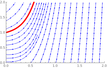
Consider an initial value problem for the first order Riccati differential equation:

\[ y'(x) = g(x) + f(y), \qquad y(x_0 ) = y_0 , \]
for polynomials g(x) and f(y) of degree at most two. Since a Riccati equation has no singular solution, the corresponding initial value problem alsways has a unique solution. Here x0 and y0 are given real numbers. Recall that a function y(x) is a solution of the given differential equation if it is continuous, has a derivative, and satisfies the differential equation identically.

Since the slope function for the Riccati equation is a polynomials, its solution is a holomorphic function in some neighborhood of the initial point where the initial condition is specified; so it is natural to seek it in teh form of a power series:

\[ y(x) = c_0 + c_1 \left( x- x_0 \right) + c_2 \left( x- x_0 \right)^2 + c_3 \left( x- x_0 \right)^3 + \cdots = \sum_{n\ge 0} c_n \left( x- x_0 \right)^n , \quad\mbox{with } c_0 = y\left( x_0 \right) . \tag{\ref{EqFirst.3}} \]
It is natural to ask whether the above series converges, in what domain, and how to find its coefficients. It is known that a power series converges within a circle \( \left\vert x- x_0 \right\vert < R , \) for some not negative number R. If R = 0, the power series diverges. The radius of convergence is the distance to the nearest singular point for sum-function. Generally speaking, it is very hard (or even impossible) to determine the radius of convergence because you have to determine (or estimate) all coefficients
\begin{equation} \label{EqFirst.7}
R^{-1} = \limsup_{n\to \infty} \sqrt[n]{\left\vert c_n \right\vert} = \lim_{n\to \infty} \left\vert \frac{c_{n+1}}{c_n} \right\vert , \end{equation}
or at least to know how they grow. Since the solution function y(x) is unknown, our task is to find a way to determine the coefficients cn of the power series, which is usually called the Taylor series. These coefficients are obtained upon calculating the derivatives:
\[ c_n = \frac{1}{n!}\, y^{(n)} (x_0 ) , \qquad n=0,1,2,\ldots . \]
At first glance, it seems that Taylor's series is an ideal tool for solving initial value problems because we need to know only infinitesimal behavior of the solution y(x) at one point---the center of the series. In principle, we can find all derivatives of the slope function at the initial point. However, it requires differentiation of the composition function f(x, y(x)) with respect to independent variable x, for which the corresponding formula is known---it is the famous Faà di Bruno's formula. Unfortunately, the number of terms in this formula grows exponentially (except some simple slope functions), and it becomes intractable. Another problem with Taylor's series representation is determination of its radius of convergence. Although we know that it should be a distance to a nearest singular point, but how to find this point can be very challengeable problem. Moreover, nonlinear differential equations may have not only fixed singular points but also moving singular points.


Another option to find a Taylor series representation is to substitute the power series \( y(x) = \sum_{n\ge 0} c_n \left( x - x_0 \right)^n \) into the given equation \( y' = f(x,y) \) and equate the coefficients of like power terms.


We demonstrate how the power series works for solving initial value problems in in the lump of examples.


Example: We start with the standard Riccati equation, which solution was found previously, in section, and perform all operations in hope that all calculations become transparent. So we consider the initial value problem

\[ y'(x) = x^2 + y^2 (x) , \qquad y(0)=0. \]
Its solution is known to be
\[ y(x) = x\,\frac{Y_{-3/4} \left( \frac{x^2}{2} \right) - J_{-3/4} \left( \frac{x^2}{2} \right)}{Y_{1/4} \left( \frac{x^2}{2} \right) -J_{1/4} \left( \frac{x^2}{2} \right) } = \frac{x^3}{3} + \frac{1}{63}\, x^7 + \frac{2}{2079}\,x^{11} + \cdots . \]
AsymptoticDSolveValue[{y'[x] == x^2 + (y[x])^2 , y[0] == 0}, y[x], {x, 0, 15}]
x^3/3 + x^7/63 + (2 x^11)/2079 + (13 x^15)/218295
We first explore the option of determination of Taylor's coefficients in the solution \( y(x) = \sum_{n\ge 0} c_n \, x^n . \) The initial term in its power series is obviously zero to match the initial condition y(0) = 0. The first coefficient is
\[ c_1 = y' (0) = f(0,0) = 0^2 + 0^2 =0 \]
because the slope function is \( f(x,y) = x^2 + y^2 . \) Now we calculate the second coefficient:
\[ c_2 = \frac{1}{2}\,y'' (0) = \left. \frac{1}{2}\, \frac{\partial \left( x^2 + y^2 (x) \right)}{\partial x} \right\vert_{x=0, y=0} = \left. \frac{1}{2}\left[ 2x + 2y\, y' \right] \right\vert_{x=0, y=0} = 0. \]
The third coefficient is
\[ c_3 = \frac{1}{3!}\,y''' (0) = \left. \frac{1}{3!}\, \frac{\partial^2 \left( x^2 + y^2 (x) \right)}{\partial x^2} \right\vert_{x=0, y=0} = \left. \frac{1}{3}\, \frac{\partial \left( x + y (x)\, y' (x) \right)}{\partial x^2} \right\vert_{x=0, y=0} = \frac{1}{3}\left[ 1 + \left( y' (x) \right)^2 + y(x)\, y'' (x) \right]_{x=0, y=0} = \frac{1}{3} . \]
For the fourth coefficient, we need to find the third derivative of the slope function:
\[ \frac{\partial^3 \left( x^2 + y^2 (x) \right)}{\partial x^3} = 6\, y' (x)\,y'' (x) + 2\, y(x)\,y''' (x) . \]
Of course, we check with Mathematica
D[x^2 + u[x]^2, {x, 3}]
6 u'[x] u''[x] + 2 u[x] u^(3)[x]
Since initially, the solution and its derivative are zeroes, we get c4 = 0. Next coefficients is very hard to obtain manually, and application of a computer algebra system is appreciated. However, complexity of operations grows as a show ball.


Now we explore the second option and substitute the power series \( y(x) = \sum-{n\ge 1} c_n \,x^n \) into the differential equation. Since its first derivative is
\[ y' (x) = \sum_{n\ge 1} c_n \,n \,x^{n-1} = \sum_{k\ge 0} c_{k+1} \left( k+1 \right) x^k , \]
we obtain
\[ \sum_{k\ge 0} c_{k+1} \left( k+1 \right) x^k = x^2 + \left( \sum_{n\ge 1} c_n \,x^{n} \right)^2 . \]
Since the product of two series leads to the convolution
\[ \left( \sum_{n\ge 1} c_n \,x^{n} \right)^2 = \sum_{n\ge 1} b_n \,x^{n} , \]
where
\[ b_n = \sum_{k=1}^n c_k c_{b-k} , \]
we get the equation between two series
\[ \sum_{n\ge 0} c_{n+1} \left( n+1 \right) x^n = x^2 + \sum_{n\ge 1} b_n \,x^{n} . \]
Equating coefficients of like powers, we obtain
\[ \begin{array}{clcl} x^0 : & c_1 = 0 & \Longrightarrow & c_1 =0 \\ x^1 : & 2\,c_2 = 0 & \Longrightarrow & c_2 = 0 \\ x^2 : & 3\,c_3 = 1 + c_1^2 & \Longrightarrow & c_3 = 1/3 \\ x^3 : & 4\, c_4 = 2\,c_1 c_2 & \Longrightarrow & c_4 = 0 \\ x^4 : & 5\, c_5 = 2\,c_1 c_3 + c_2^2 & \Longrightarrow & c_5 = 0 \\ x^5 : & 6\,c_6 = 2\,c_1 c_4 + 2\,c_2 c_3 & \Longrightarrow & c_6 = 0 \\ x^6 : & 7\,c_7 = 2\,c_1 c_5 + 2\,c_2 c_4 + c_3^2 & \Longrightarrow & c_7 = 1/63 \end{array} \]
and so on. Now we demonstrate the Frobenius method by substituting the power series \( y = \sum_{n\ge 1} c_n x^n \) into the given Riccati equation.
\[ \sum_{n\ge 1} c_{n+1} \left( n+1 \right) x^n = x^2 + \sum_{k\ge 1}^n c_k c_{n-k} \,x^n . \]
Equating the like powers of x yields the full-history recurrence:
\[ c_{n+1} \left( n+1 \right) = \delta_{n,2} + \sum_{k\ge 1}^n c_k c_{n-k} , \qquad n=1,2,\ldots , \]
where δ is the Kronecker delta. We immediately find c1 = 0 and for other terms:
\[ c_{n+1} = \frac{1}{n+1} \left[ \delta_{n,2} + \sum_{k\ge 1}^n c_k c_{n-k} \right] , \qquad n=1,2,\ldots . \]
   ■

Example: Consider the initial value problem for the Riccati equation

\[ y' = 8\,x^2 + \frac{1}{2}\, y^2 , \qquad y(0) = 1. \]
     
field = StreamPlot[{1, 8*x^2 + (1/2)*y^2}, {x, 0, 2}, {y, 0, 2}, StreamStyle -> Blue, FrameStyle -> Arrowheads[0.02], Background -> LightGreen, PerformanceGoal -> "Quality", StreamPoints -> 20];
sol = Simplify[DSolve[{y'[x] == 8*x^2 + (1/2)*(y[x])^2, y[0] == 1}, y[x], x]]
{{y[x] -> (-4 x^2 BesselJ[-(3/4), x^2] Gamma[1/4] + 4 Sqrt[2] (2 x^2 BesselJ[-(5/4), x^2] + BesselJ[-(1/4), x^2] - 2 x^2 BesselJ[3/4, x^2]) Gamma[3/ 4])/(x (BesselJ[1/4, x^2] Gamma[1/4] - 4 Sqrt[2] BesselJ[-(1/4), x^2] Gamma[3/4]))}}
curve = Plot[Evaluate[y[x] /. sol], {x, 0, 0.6}, PlotRange -> {{0, 2}, {0, 2}}, PlotStyle -> {Red, Thickness[0.013]}];
Show[curve, field]
       Direction field and the solution.            Mathematica code

Its explicit solution for x > 0 is
\begin{align*} y(x) &= \frac{-4x^2 J_{-3/4} \left( x^2 \right) \Gamma\left( \frac{1}{4} \right) + 4\sqrt{2} \left[ 2x^2 J_{-5/4} \left( x^2 \right) + J_{-1/4} \left( x^2 \right) -2x^2 J_{3/4} \left( x^2 \right) \right] \Gamma\left( \frac{3}{4} \right)}{x \left[ J_{1/4} \left( x^2 \right) \Gamma\left( \frac{1}{4} \right) -4\sqrt{2} J_{-1/4} \left( x^2 \right) \Gamma\left( \frac{3}{4} \right) \right]} \\ &= -4x\,\frac{\left( \pi \sqrt{2} - 4\,\Gamma^2 \left( \frac{3}{4} \right) \right) J_{-3/4} \left( x^2 \right) + 4\,Y_{-3/4} \left( x^2 \right) \Gamma^2 \left( \frac{3}{4} \right)}{\left( \pi \sqrt{2} - 4\,\Gamma^2 \left( \frac{3}{4} \right) \right) J_{1/4} \left( x^2 \right) + 4\,Y_{1/4} \left( x^2 \right) \Gamma^2 \left( \frac{3}{4} \right)} . \end{align*}
      Two formulas above are equivalent: they were found with the aid of Mathematica and Maple. Upon plotting the denominator
denom[x_] = x*(BesselJ[1/4, x^2] Gamma[1/4] - 4 Sqrt[2] BesselJ[-(1/4), x^2] Gamma[3/4]);
Plot[denom[x], {x, 0, 2}, PlotStyle -> {Purple, Thickness[0.015]}]
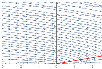
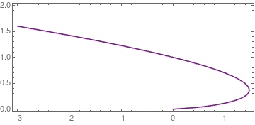
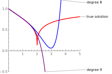
we see that the solution blows up at x = 1.219762884 where the denominator is zero. It is impossible to determine this singularity from the power series
AsymptoticDSolveValue[{y'[x] == 8*x^2 + (1/2)*(y[x])^2, y[0] == 1}, y[x], {x, 0, 10}]
1 + x/2 + x^2/4 + (67 x^3)/24 + (35 x^4)/48 + (69 x^5)/160 + ( 239 x^6)/960 + (26171 x^7)/40320 + (3267 x^8)/8960 + ( 39803 x^9)/161280 + (28687 x^10)/179200
       Plot of the denominator.            Mathematica code

\[ y(x) = 1 + \frac{x}{2} + \frac{x^2}{4} + \frac{67}{24}\, x^3 + \frac{35}{48} \, x^4 + \frac{69}{160}\, x^5 + \frac{239}{960}\, x^6 + \frac{26171}{40320}\, x^7 + \frac{3267}{8960} \, x^8 + \cdots . \]
      We plot the true solution and its eighth degree polynomial approximation.
sol = Simplify[ DSolve[{y'[x] == 8*x^2 + (1/2)*(y[x])^2, y[0] == 1}, y[x], x]];
Plot[{Callout[Evaluate[y[x] /. sol], "true solution"] , Callout[1 + x/2 + x^2/4 + (67 x^3)/24 + (35 x^4)/48 + (69 x^5)/160 + (239 x^6)/ 960 + (26171 x^7)/40320 + (3267 x^8)/8960 + (39803 x^9)/ 161280 + (28687 x^10)/179200, "Polynomial approximant"]}, {x, 0, 1.1}, PlotRange -> {{0, 1.1}, {0.8, 10.2}}, PlotStyle -> {Thickness[0.013]}]
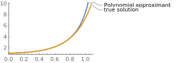
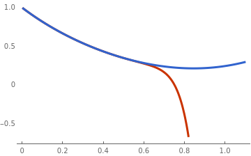
       True solution along with the polynomial approximation.            Mathematica code

We first apply the Taylor series method to determine the coefficients in the expression above. Assuming that the solution can be obtained as a Taylor series
\[ y(x) = 1 + x\,y' (0) + \frac{x^2}{2!}\, y'' (0) + \frac{x^3}{3!}\, y''' (0) + \]
we find
\begin{align*} y' (0) &= \lim_{x\to 0} \, \left\{ 8\,x^2 + \frac{1}{2}\,y^2 (x) \right\} = \frac{1}{2}\,y^2 (0) = \frac{1}{2} , \\ y'' (0) &= \lim_{x\to 0} \, \frac{\text d}{{\text d}x} \left\{ 8\,x^2 + \frac{1}{2}\,y^2 (x) \right\} =\lim_{x\to 0} \, \left\{ 16\,x + y(x)\, y' (x) \right\} = y' (0) = \frac{1}{2} , \\ y''' (0) &= \lim_{x\to 0} \,\frac{\text d}{{\text d}x} \left\{ 16\,x + y(x)\, y' (x) \right\} = \lim_{x\to 0} \,\left\{ 16 + y'(x)\, y' (x) + y(x)\, y'' (x) \right\} = 16 + \frac{1}{2}\,\frac{1}{2} + \frac{1}{2} = \frac{67}{4} , \end{align*}
and so on.

Using Mathematica, we find the solution of the same Riccati equation under another initial conditions

sol2 = Simplify[ DSolve[{y'[x] == 8*x^2 + (1/2)*(y[x])^2 , y[0] == 1/2}, y[x], x]]
{{y[x] -> (-4 x^2 BesselJ[-(3/4), x^2] Gamma[1/4] + 8 Sqrt[2] (2 x^2 BesselJ[-(5/4), x^2] + BesselJ[-(1/4), x^2] - 2 x^2 BesselJ[3/4, x^2]) Gamma[3/ 4])/(x (BesselJ[1/4, x^2] Gamma[1/4] - 8 Sqrt[2] BesselJ[-(1/4), x^2] Gamma[3/4]))}}
This solution
\[ y(x) = \frac{- 4\,x^2 J_{-3/4} \left( x^2 \right) \Gamma \left( \frac{1}{4} \right) + 8\sqrt{2} \left[ 2x^2 J_{-5/4} \left( x^2 \right) + J_{-1/4} \left( x^2 \right) - x^2 J_{3/4} \left( x^2 \right) \right] \Gamma \left( \frac{3}{4} \right)}{x \left[ J_{1/4} \left( x^2 \right) \Gamma \left( \frac{1}{4} \right) - 8\,\sqrt{2}\, J_{-1/4} \left( x^2 \right) \Gamma \left( \frac{3}{4} \right) \right]} , \qquad y(0) = \frac{1}{2} , \]
blows up at x = 1.337033790, where the denominator vanishes.
FindRoot[ (x (BesselJ[1/4, x^2] Gamma[1/4] - 8 Sqrt[2] BesselJ[-(1/4), x^2] Gamma[3/4])) == 0, {x, 1}]
{x -> 1.3370337902385145}
Similarly, we can find a solution of the given Riccati equation under the homogeneous initial condition
\[ y(x) = -4x\, \frac{J_{-3/4} \left( x^2 \right) - Y_{-3/4} \left( x^2 \right)}{J_{1/4} \left( x^2 \right) - Y_{1/4} \left( x^2 \right)} , \qquad y(0) = 0 . \]
FindRoot[BesselJ[1/4, x^2] == BesselY[1/4, x^2], {x, 1.3}]
{x -> 1.4164390815666765}
This function blows up at x = 1.416439082. So we see that solutions under different initial conditions blow up at different points. This indicates that their solutions have a moving singularity depending on the value of the initial condition.    ■

Example: We attack the same initial value problem \( y' = 8\, x^2 + \frac{1}{2}\,y^2 , \quad y(0) =1 , \) using a different approach.

We make a Bernoulli substitution

\[ y(x) = u^r v^s \]
and hope to be able to choose functions u(x), v(x), and parameters r, s in order to transfer the given Riccati equation into two separable equations, one for function u(x) along and another one for v(x).

Using its derivative

\[ y'(x) = \left( u^r \right)' v^s + u^r \left( v^s \right)' = r\,u^{r-1} u' (x)\, v^s + u^{r} s\,v^{s-1} v' (x) , \]
we substitute the product into the Riccati equation to obtain
\[ r\,u^{r-1} u' (x)\, v^s + u^{r} s\,v^{s-1} v' (x) = 8\,x^2 + \frac{1}{2} \, u^{2r} v^{2s} . \]
Choosing
\[ \begin{split} r\,u^{r-1} u' (x)\, v^s &= 8\,x^2 , \\ u^{r} s\,v^{s-1} v' (x) &= \frac{1}{2} \, u^{2r} v^{2s} \end{split} \]
we get from the latter that
\[ u^{r} s\,v^{s-1} v' (x) = \frac{1}{2} \, u^{2r} v^{2s} \qquad \Longrightarrow \qquad s\, v' (x) = \frac{1}{2} \,u^{r} v^{s+1} . \]
The non-linearity can be removed by choosing s = -1, so the equation becomes
\[ v' (x) = - \frac{1}{2} \,u^{r} \qquad \Longrightarrow \qquad v'' (x) = - \frac{1}{2} \left( u^{r} \right)' = - \frac{1}{2} \,8x^2\,v . \]
Therefore, the function v(x) must be a solution of the second order differential equation
\[ v'' + 4\,x^2 v = 0 , \]
which is a Bessel equation. Since \( u^{r} = -2\, v' (x) , \) we obtain the required transformation
\[ y (x) = - 2\,\frac{v'}{v} , \qquad \mbox{where} \quad v(x) = C_1 \sqrt{x}\,J_{1/4} \left( x^2 \right) + C_2 \sqrt{x}\,Y_{1/4} \left( x^2 \right) , \]
with some arbitrary constants C1, C2. As usual, Jν and Yν denote the Bessel functions of the first and second kind, respectively.

We find the Taylor series solution \( v(x) = \sum_{n\ge 0} c_n x^n \) of the differential equation \( v'' + 4\,x^2 v = 0 . \) . Its substitution into the differential equation yields

\[ \sum_{n\ge 2} c_n n \left( n-1 \right) x^{n-2} + 4\, \sum_{n\ge 0} c_n x^{n+2} = 0. \]
This gives us the fourth order difference equation:
\[ \left( n+2 \right) \left( n+1 \right) c_{n+2} = - 4\, c_{n-2} , \qquad n= 2,3, \ldots . \]
Since c2 = 0, c3 = 0, we have
\[ c_{n+4} = - \frac{4}{(n+3)(n+4)}\, c_n , \qquad n = 0,1,2,\ldots . \]
This allows us to determine the first few terms in the Taylor series:
\[ v(x) = c_0 \left[ 1 + \frac{x^4}{3} + \frac{x^8}{42} + \frac{x^{12}}{1386} + \frac{x^{16}}{83160} + \cdots \right] + c_1 \left[ x - \frac{x^5}{5} + \frac{x^9}{90} - \frac{x^{13}}{3510} + \frac{x^{17}}{238680} - \cdots \right] , \]
where c0 = v(0) and c1 = v'(0) are the initial values that play the role of arbitrary constants.

⊛ Although we found the general solution as a ratio of two power series, it is far away from the required series representation because we need identify the values of the constant k = c1/c0 and the divide the two power series. Instead, we use another approach and introduce the function

\[ p(x) = \frac{x}{y(x)} \qquad \Longrightarrow \qquad |p(x) | \le 1. \]
First, we calculate
\[ \frac{\text d}{{\text d}x} \left( - \frac{1}{y} \right) = \frac{y' (x)}{y^2 (x)} = \frac{8\,x^2 + y^2 /2}{y^2} = 8\,\frac{x^2}{y^2} + \frac{1}{2} = 8\,p^2 + \frac{1}{2} . \tag{A} \]
Starting with p = 0, we get
\[ \frac{\text d}{{\text d}x} \left( - \frac{1}{y} \right) = \frac{1}{2} \qquad \Longrightarrow \qquad - \frac{1}{y} = K + \frac{x}{2} , \qquad \mbox{$K$ is a constant} . \]
The condition y(0) = 1 yields K = -1 and we have the first approximation
\[ \frac{1}{y} = 1 - \frac{x}{2} , \qquad \Longrightarrow \qquad \phi_1 (x) = \frac{1}{1 - x/2} = 1 + \frac{x}{2} + \frac{x^2}{4} + \cdots . \]
Second estimate: As a reciprocal of y, we get
\[ p = \frac{x}{y} = x - \frac{x^2}{2} . \]
Integrating equation (A) with this expression for p yields
\[ -\frac{1}{y} = -1 + \int_0^x \left( 8\, p^2 + \frac{1}{2} \right) {\text d} x = -1 + \frac{x}{2} + \frac{8}{3}\, x^3 - 2\,x^4 + \frac{2}{5}\, x^5 . \]
Integrate[8*(s - s^2 /2)^2 + 1/2, {s, 0, x}]
x/2 + (8 x^3)/3 - 2 x^4 + (2 x^5)/5
The second approximant for p becomes
\[ p_2 = \frac{x}{y} = -x \left( -1 + \frac{x}{2} + \frac{8}{3}\, x^3 - 2\,x^4 + \frac{2}{5}\, x^5 \right) . \]
Then its reciprocal gives the second approximant to the solution:
\[ \phi_2 (x) = \frac{x}{p(x)} = \frac{-1}{-1 + \frac{x}{2} + \frac{8}{3}\, x^3 - 2\,x^4 + \frac{2}{5}\, x^5} = {\bf 1 + \frac{x}{2} + \frac{x^2}{4} + \frac{67}{24}\, x^3 + \frac{35}{48}\, x^4 + \frac{69}{160}\, x^5 } + \frac{21197}{2880} \, x^6 + \cdots , \]
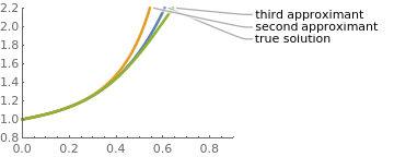
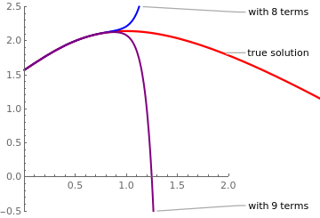
with first five correct terms. Note that the solution to the given initial value problem has a singularity at x = 1.219762884. Therefore, we expect that ϕ2(x) gives better approximation.
Series[-1/(-1 + x/2 + (8 x^3)/3 - 2 x^4 + (2 x^5)/5), {x, 0, 9}]
SeriesData[x, 0, {1, Rational[1, 2], Rational[1, 4], Rational[67, 24], Rational[35, 48], Rational[69, 160], Rational[21197, 2880], Rational[271, 1920], Rational[225, 256], Rational[1347527, 69120]}, 0, 10, 1]
Indeed, the polynomial in the denominator of ϕ2(x) vanishes at x = 0.766669.
FindRoot[-1 + x/2 + (8 x^3)/3 - 2 x^4 + (2 x^5)/5 == 0, {x, 1.0}]
{x -> 0.766669}
Third estimate: With \( \displaystyle p = -x \left( -1 + \frac{x}{2} + \frac{8}{3}\, x^3 - 2\,x^4 + \frac{2}{5}\, x^5 \right) , \) we integrate again and obtain
\[ - \frac{1}{y} = -1 + \int_0^x \left( 8\, p^2 + \frac{1}{2} \right) {\text d} x = -1 + \frac{x}{2} + \frac{8}{3}\, x^3 - 2\,x^4 + \frac{2}{5}\, x^5 - \frac{64}{9}\, x^6 + \frac{160}{21}\, x^7 - \frac{14}{5}\, x^8 + \frac{2704}{405}\, x^9 - \frac{128}{15}\, x^{10} + \frac{736}{165}\, x^{11} - \frac{16}{15}\, x^{12} + \frac{32}{325}\, x^{13} . \]
Integrate[ s^2 *8*(-1 + s/2 + (8 s^3)/3 - 2 s^4 + (2 s^5)/5 )^2 + 1/2, {s, 0, x}]
x/2 + (8 x^3)/3 - 2 x^4 + (2 x^5)/5 - (64 x^6)/9 + (160 x^7)/21 - ( 14 x^8)/5 + (2704 x^9)/405 - (128 x^10)/15 + (736 x^11)/165 - ( 16 x^12)/15 + (32 x^13)/325
Hence, the third approximant to the required solution is
\[ \phi_3 (x) = \frac{-1}{-1 + \frac{x}{2} + \frac{8}{3}\, x^3 - 2\,x^4 + \frac{2}{5}\, x^5 - \frac{64}{9}\, x^6 + \frac{160}{21}\, x^7 - \frac{14}{5}\, x^8 + \frac{2704}{405}\, x^9 - \frac{128}{15}\, x^{10} + \frac{736}{165}\, x^{11} - \frac{16}{15}\, x^{12} + \frac{32}{325}\, x^{13}} . \]
The denominator vanishes at x = 1. 026.
FindRoot[ -1 + x/2 + (8 x^3)/3 - 2 x^4 + (2 x^5)/5 - (64 x^6)/9 + ( 160 x^7)/21 - (14 x^8)/5 + (2704 x^9)/405 - (128 x^10)/15 + ( 736 x^11)/165 - (16 x^12)/15 + (32 x^13)/325 == 0, {x, 1}]
{x -> 1.026}
      Finally, we compare the explicit solution y(x) along with two rational approximants:
sol = Simplify[ DSolve[{y'[x] == 8*x^2 + (1/2)*(y[x])^2, y[0] == 1}, y[x], x]];
phi2[x_] = -1/(-1 + x/2 + (8 x^3)/3 - 2 x^4 + (2 x^5)/5);
phi3[x_] = (-1)/(-1 + x/2 + (8 x^3)/3 - 2 x^4 + (2 x^5)/5 - (64 x^6)/ 9 + (160 x^7)/21 - (14 x^8)/5 + (2704 x^9)/405 - (128 x^10)/15 + ( 736 x^11)/165 - (16 x^12)/15 + (32 x^13)/325);
Plot[{Callout[Evaluate[y[x] /. sol], "true solution"] , Callout[phi2[x], "second approximant"], Callout[phi3[x], "third approximant"], Below}, {x, 0, 0.8}, PlotRange -> {{0, 0.9}, {0.8, 2.2}}, PlotStyle -> {Thickness[0.013]}]
       True solution and two approximants.            Mathematica code

   ■

Example: Our next example shows how to handle the differential equation with the rational slope. Consider the initial value problem

\[ \frac{{\text d}y(x)}{{\text d}x} = \frac{y (x)}{x - 4\,y(x)} , \qquad y(0) =1. \]
Its solution exists in the interval (-∞, 4/e) ≈ (-∞, 1.47152) because it is the implicit solution of the equation \( y\,\ln |y| + x/4 = 0 , \) which is expressed through the Lambert function. It has the following power series expansion:
\[ y(x) = 1 - \frac{x}{4} - \frac{x^2}{32} - \frac{x^3}{96} - \frac{9}{2048}\,x^4 - \frac{1}{480}\, x^5 - \frac{81}{143 360}\, x^7 - \frac{117 649}{377 487 360}\, x^8 - \cdots . \]
The first two coefficients in the power series \( y(x) = \sum_{n\ge 0} c_n \,x^n \) immediately follow from the initial conditions:
\[ c_0 = y(0) = 1 , \qquad c_1 = y' (0) = f(0,1) = -\frac{1}{4} , \]
where \( f(x,y) = \frac{y}{x-4y} \) is the slope function. Its first few derivatives are
\begin{align*} \frac{{\text d} f(x,y)}{{\text d}x} &= \frac{\partial f(x,y)}{\partial x} + \frac{\partial f(x,y)}{\partial y} \,y' (x) = \frac{-y}{(x-4y)^2} + \frac{xy}{(x-4y)^3} , \\ \frac{{\text d}^2 f(x,y)}{{\text d}x^2} &= \frac{{\text d}}{{\text d}x} \left( \frac{xy}{(x-4y)^3} - \frac{y}{(x-4y)^2} \right) = \frac{8y^2 \left( x+ 2y \right)}{(x-4y)^5} - \frac{12\, y^2}{(x-4y)^4} \end{align*}
f[x_, y_] = y/(x - 4*y)
D[f[x, y], {x}]
-(y/(x - 4 y)^2)
Therefore,
\[ c_2 = \left. \frac{1}{2!}\,\frac{{\text d} f(x,y)}{{\text d}x} \right\vert_{x=0,y=1} = - \frac{1}{32} , \qquad c_3 = \left. \frac{1}{3!}\,\frac{{\text d}^2 f(x,y)}{{\text d}x^2} \right\vert_{x=0, y=1} = - \frac{1}{96} . \]
(D[f[x, y], {y}]*f[x, y] + D[f[x, y], {x}]) /. {x -> 0, y -> 1} D[D[f[x, y], {y}]*f[x, y] + D[f[x, y], {x}],x] /. {x -> 0, y -> 1} D[D[f[x, y], {y}]*f[x, y] + D[f[x, y], {x}],y]*f[x, y] /. {x -> 0, y -> 1}
Now we plot a corresponding direction field and the true solution.
ContourPlot[y*Log[y] + x/4 == 0, {x, -3, 1.47}, {y, 0, 2}, AspectRatio -> Automatic, ContourShading -> Automatic, ColorFunction -> "Rainbow"]
stream = StreamPlot[{1, y/(x - y*4)}, {x, -3, 2.5}, {y, 0, 5}, MeshShading -> {LightOrange, Black}, MeshStyle -> {Thick}, VectorPoints -> Automatic]
line = Plot[x/4, {x, -3, 2.6}, PlotStyle -> {Thick, Red}, PlotRange -> {{-3, 2.5}, {0, 5}}]
Show[line, stream]
         Stream plot       Solution curve
   ■

Example: Consider the initial value problem for the autonomous equation of the first order:

\[ y'(x)+y^2 (x)=1, \qquad y(0)=0. \]
The differential equation has two equilibrium solutions: y = 1 is asymptotically stable, while y = -1 is unstable.
VectorPlot[{1, 1 - y^2}, {x, 0, 2}, {y, -2, 2}, VectorScale -> {Small, Automatic, None}, VectorColorFunction -> Hue, VectorPoints -> 14]
         Direction field.       Mathematica code.

The given initial value problem has the closed-form solution
\[ y(x) = \tanh (x) = x - \frac{x^3}{3} + \frac{2x^5}{5} - \frac{17}{315}\, x^7 - \cdots . \]
This series converges for 0 ≤ x < 3/2. However, by means of exponential functions as basis this function has another expansion
\[ y(x) = \tanh (x) = 1+ \lim_{m\to +\infty} \left[ 2 \sum_{n=1}^m (-1)^ne^{-2nx} +(-1)^{m+1} e^{-(2+1)x} \right] , \]
that converges to the exact solution for all 0 ≤ x < +∞.


⏧ Application of the Taylor series method yields
\begin{align*} y'(0) &= \lim_{x\to 0} \left[ 1 - y^2 (x) \right] = 1 - y^2 (0) = 1 , \\ y''(0) &= \lim_{x\to 0} \frac{\text d}{{\text d}x} \left[ 1 - y^2 (x) \right] = \lim_{x\to 0} \left[ -2y(x)\, y' (x) \right] = -2\cdot 0 \cdot 1 = 0 , \\ y'''(0) &= \lim_{x\to 0} \frac{{\text d}^2}{{\text d}x^2} \left[ 1 - y^2 (x) \right] = \lim_{x\to 0} \frac{\text d}{{\text d}x} \left[ -2y(x)\, y' (x) \right] = \lim_{x\to 0} \left[ - 2\,y' (x)\,y'(x) -2y(x)\, y'' (x) \right] = -2, \\ y^{(4)}(0) &= \lim_{x\to 0} \frac{\text d}{{\text d}x} \left[ - 2\,y' (x)\,y'(x) -2y(x)\, y'' (x) \right] = \lim_{x\to 0} \left[ - 6\,y' (x)\,y''(x) -2y(x)\, y''' (x) \right] = 0 , \end{align*}
and so on. Thus, we see that the number of terms needed to evaluate derivatives grow exponentially.


⊛ Now we use the Frobenius method and derive the coresponding recurrence relation for coefficients of the solution:
\[ y(x) = \sum_{n\ge 0} c_n x^n , \qquad c_0 = 0 . \]
Substituting the series into the differential equation, we get
\[ \sum_{n\ge 1} c_n n\, x^{n-1} = \sum_{n\ge 0} c_{n+1} \left( n+1 \right) x^n = 1 - \sum_{n\ge 0} \left[ \sum_{k=0}^n c_k c_{n-k} \right] x^n . \]
Equating coefficients of like powers of x, we obtain the full-history recurrence:
\[ \begin{cases} c_0 = 0, & \quad n=0, \\ c_1 = 1 , & \quad n=1, \\ c_{n+1} = \frac{-1}{n+1} \,\sum_{k=0}^n c_k \, c_{n-k} & \quad n=1,2,\ldots . \end{cases} \]
   ■

Example: Consider the initial value problem for a separable equation of the first order:

\[ (4-x^2 )y'(x)+y(x)=0, \qquad y(0)=1. \]
The differential equation has two singular points: x = ±2.
field = StreamPlot[{1, y/(x^2 - 4)}, {x, -5, 5}, {y, -2, 2}, StreamColorFunction -> "Rainbow", StreamPoints -> 40, StreamScale -> {Full, All, 0.04}];
curv[x_] = Abs[2 - x]^(1/4)/Abs[2 + x]^(1/4);
cu = Plot[curv[x], {x, 0, 5}, PlotStyle -> {Red, Thickness[0.01]}];
Show[field, cu]
The first few terms in the power series solution can be obtained with the aid of Mathematica:
AsymptoticDSolveValue[{(4 - x^2)*y'[x] + y[x] == 0, y[0] == 1}, y[x], {x, 0, 10}]
1 - x/4 + x^2/32 - (3 x^3)/128 + (11 x^4)/2048 - (31 x^5)/8192 + ( 69 x^6)/65536 - (187 x^7)/262144 + (1843 x^8)/8388608 - ( 4859 x^9)/33554432 + (12767 x^10)/268435456
         Direction field.       Mathematica code.

The Taylor series method quickly becomes a mess because we need to differentiate the slope function

\[ f(x,y) = \frac{y}{x^2 -4} , \qquad x \ne \pm 2. \]
Instead, we derive a recurrence relation for its power series solution:
\[ y(x) = \sum_{n\ge 0} c_n x^n , \qquad c_0 = 1. \]
Product of (4 - x²) and the derivative of y(x) gives
\[ \left( 4 - x^2 \right) y' (x) = 4 \,\sum_{n\ge 1} c_n n\, x^{n-1} - \sum_{n\ge 1} c_n n\, x^{n+1} = 4\, \sum_{n\ge 0} c_{n+1} \left( n+1 \right) x^n - \sum_{n\ge 1} c_{n-1} \left( n-1 \right) x^n . \]
This allows us to derive the recurrence:
\[ 4\,c_{n+1} \left( n+1 \right) - c_{n-1} \left( n-1 \right) + c_n = 0, \qquad n=1,2,\ldots . \]
With c1 = -1/4, we obtain the second order difference equation:
\[ c_{n+1} = - \frac{1}{4\,(n+1)} \, c_n + \frac{n-1}{4\,(n+1)} \, c_{n-1} , \qquad n=1,2,\ldots . \]
Clear[a,n]
a[n_]:=a[n]=((n-2) a[n-2] -a[n-1])/4/n
a[0] = a0
a[1] = -a0/4
TableForm[Table[{n,a[n]},{n,0,5}]]
Out[21]/TableForm=
0 a0
1 -a0/4
2 a0/32
3 -3 a0/128
4 11 a0/2048
5 -31 a0/8192

When we apply the initial condition, we set a0=1 in the general solution.

Now we solve the initial value problem exactly:

Clear[x,y]
exactsol=DSolve[{(4-x^2)y'[x]+y[x]==0,y[0]==1},y[x],x]
Out[63]= {{y[x]-> (2-x)^(1/4)/(2+x)^(1/4) }}
Note that the exact solution is
\[ y(x) = \left( \frac{|2-x|}{|2+x|} \right)^{1/4} \]
with absolute values instead of parenthethis.

We plot the true solution along with two polynomials of degree 8 and 9:

poly8[x_] = 1 - x/4 + x^2/32 - (3 x^3)/128 + (11 x^4)/2048 - (31 x^5)/8192 + ( 69 x^6)/65536 - (187 x^7)/262144 + (1843 x^8)/8388608;
poly9[x_] = 1 - x/4 + x^2/32 - (3 x^3)/128 + (11 x^4)/2048 - (31 x^5)/8192 + ( 69 x^6)/65536 - (187 x^7)/262144 + (1843 x^8)/8388608 - (4859 x^9)/ 33554432;
curv[x_] = Abs[2 - x]^(1/4)/Abs[2 + x]^(1/4);
Plot[{Callout[curv[x], "true solution"], Callout[poly8[x], "degree 8"], Callout[poly9[x], "degree 9"]}, {x, 0, 5}, AspectRatio -> 1, PlotRange -> {{0, 5}, {-0.5, 1.2}}, PlotStyle -> {{Red, Thickness[0.01]}, {Blue, Thick}, {Purple, Thick}}]
         True solution (in red) and its two polynomial approximations.       Mathematica code.

Note that the exact solution is |2-x|^(1/4)/|2+x|^(1/4) with absolute values instead of parenthesis.

formula=Simplify[(2-x)^(1/4)/(2+x)^(1/4)]
Out[64]= (2 - x)^(1/4)/(2 + x)^(1/4)
var=Table[D[y[x],i]/.x->0,{i,1,11}]
????sols=Solve[sysofeqs,vars]
sersol=Series[y[x],{x,0,11}/.sols[[1]]]

   ■

Example: Consider the differential equation with a sinusoidal nonlinearity

\[ y' = \sin \left( y(x) + x \right) , \qquad y(0) = \pi /2. \]
The direction field along with the true solution (in orange):
field = StreamPlot[{1, Sin[x + y]}, {x, -5, 5}, {y, -5, 5}, StreamColorFunction -> "Rainbow", StreamPoints -> 50, StreamScale -> {Full, All, 0.04}];
curve = Plot[2 ArcCos[-((-1 + x)/Sqrt[2 + 2 x^2])] - x, {x, -0.2, 3}, PlotRange -> {{0, 3}, {1, 2.5}}, PlotStyle -> {Orange, Thickness[0.01]}];
Show[field, curve]

As this graph indicates, the equation has a discrete number of separatrix lines:    x + y = k π,     k = 0, ±1, ±2, ….

         Direction field.       Mathematica code.

Upon introducing a new variable \( u(x) = x+ y(x) , \) we reduce the equation to the autonomous one:
\[ u' = 1+\sin \left( u(x) \right) , \qquad u(0) = \pi /2. \]
Separating variables, we are able to determine the solution to the given initial value problem:
\[ y(x) = 2\,\mbox{arccos} \left( \frac{1-x}{\sqrt{2 + 2\,x^2}} \right) - x , \]
DSolve[{z'[x] == 1 + Sin[z[x]], z[0] == Pi/2}, z[x], x]
{{z[x] -> 2 ArcCos[-((-1 + x)/Sqrt[2 + 2 x^2])]}}
Next, we find its Maclaurin series with a standard Mathematica command
AsymptoticDSolveValue[{y'[x] + Sin[y[x]] == 0, y[0] == Pi/2}, y[x], {x, 0, 10}]
\[Pi]/2 - x + x^3/6 - x^5/24 + (61 x^7)/5040 - (277 x^9)/72576
\[ y(x) = \frac{\pi}{2} + x - \frac{2}{3}\, x^3 + \frac{2}{5}\, x^5 - \frac{2}{7}\, x^7 + \cdots = \frac{\pi}{2} + x + 2\sum_{n\ge 1} \frac{(-1)^n}{n}\, x^{2n+1} . \]
We plot the true solution along with two polynomials of degree 8 and 9:
poly8[x_] = 1 - x/4 + x^2/32 - (3 x^3)/128 + (11 x^4)/2048 - (31 x^5)/8192 + ( 69 x^6)/65536 - (187 x^7)/262144 + (1843 x^8)/8388608;
poly9[x_] = 1 - x/4 + x^2/32 - (3 x^3)/128 + (11 x^4)/2048 - (31 x^5)/8192 + ( 69 x^6)/65536 - (187 x^7)/262144 + (1843 x^8)/8388608 - (4859 x^9)/ 33554432;
curv[x_] = Abs[2 - x]^(1/4)/Abs[2 + x]^(1/4);
Plot[{Callout[curv[x], "true solution"], Callout[poly8[x], "degree 8"], Callout[poly9[x], "degree 9"]}, {x, 0, 5}, AspectRatio -> 1, PlotRange -> {{0, 5}, {-0.5, 1.2}}, PlotStyle -> {{Red, Thickness[0.01]}, {Blue, Thick}, {Purple, Thick}}]
         The true solution along with two polynomial approximations of order 8 and 9 respectively.       Mathematica code.

   ■

Example: Consider the initial value problem for the Abel equation

\[ y' = y^3 +x, \qquad y(0) =0. \]
Its power series solution is
\[ y(x) = \frac{x^2}{2} + \frac{x^7}{56} + \frac{x^{12}}{896} + \frac{33}{426496}\, x^{17} + \cdots . \]

We plot the separatrix and the direction field

field = StreamPlot[{1, x + y^3}, {x, -2, 2}, {y, -2, 2}, StreamColorFunction -> Hue, StreamPoints -> 42, StreamScale -> {Full, All, 0.04}];
sol = NDSolve[{y'[x] == x + (y[x])^3 , y[-2] == 1.07677}, y[x], {x, -2, 2}];
curve = Plot[Evaluate[y[x] /. sol], {x, -2, 2}, PlotRange -> {{-2, 2}, {-2, 2}}, PlotStyle -> {Blue, Thickness[0.01]}];
Show[field, curve]
         Direction field and separatrix (in blue).       Mathematica code.

We find its power series expansion using the following Mathematica commands:

y = Sum[c[i]*x^{2 + 5*i}, {i, 0, 9}] + O[x]^(48)
Out[1]= { c[0] x^2 + c[1] x^7 + c[2] x^12 + c[3] x^17 + c[4] x^22 +
c[5] x^27 + c[6] x^32 + c[7] x^37 + c[8] x^42 + c[9] x^47 +O[x]^48}
de = D[y, {x, 1}] - y^3 - x == 0;
coefeq = LogicalExpand[de];
coeffs = Solve[coefeq, Table[c[i], {0, 1, 17}]];
y = y /. coeffs
Out[5]= {{ x^2 /2 + x^7 /56 + x^12 / 896 + 33 x^17 / 426296 + 1475
x^22 / 262721536 + 879 x^27 / 2101772288 + }}

This problem can be solved in slightly different way. First, we define the differential operator (non-linear because the given equation is non-linear)

L[x_, y_] = y'[x] - x - (y[x])^3
Out[1]= -x - y[x]^3 + Derivative[1][y][x]

Then we set n to be 13, the number of terms in the power series:

n = 13
Out[2]= 13

The next cell says to create a sum of n terms and effectively turn it into a series saying that the terms beyond n are indefinite. O[x]^(n+1) indicates that we know nothing about terms of order n+1 and beyond. So we define the (finite) series

y[x_] = Sum[a[i]*x^i, {i, 0, n}] + O[x]^(n + 1)
Out[3]= a[0] + a[1] x + a[2] x^2 + a[3] x^3 + a[4] x^4 + a[5] x^5 +
a[6] x^6 + a[7] x^7 + a[8] x^8 + a[9] x^9 + a[10] x^10 + a[11] x^11 +
a[12] x^12 + a[13] x^13 + O[x]^14

Substitute this expression into the differential operator

LHS = Collect[L[x, y], x] + O[x]^n

Equate the coefficients to 0. Recall that the operator && means And.

sys = LogicalExpand[LHS == 0]

Find the coefficients a[i] in the power series of y[x] using Reverse[Table[a[i],{i,0,n}]]. The latter makes the form of the coefficients agree with what you would find by hand: the next term is expressed through the previous terms.

coeff = Solve[sys, Reverse[Table[a[j], {j, 0, n}]]]
Solve::svars: Equations may not give solutions for all "solve" variables. >>

To get the solution series, set a[0] equals to zero:

s[x_] = y[x] /. coeff[[1]] /. a[0] -> 0
Out[7]= x^2/2 + x^7/56 + x^12/896 +O[x]^14
   ▣


How to determine a polynomial approximation to the solution with CAS


Mathematica has a standard command to represent the solution in power series form. For example,

AsymptoticDSolveValue[{y''[x] + x*y'[x] + y[x] == 0, y'[0] == 2, y[0] == 1}, y[x], {x, 0, 10}]
1 + 2 x - x^2/2 - (2 x^3)/3 + x^4/8 + (2 x^5)/15 - x^6/48 - ( 2 x^7)/105 + x^8/384 + (2 x^9)/945 - x^10/3840
As you see, in a blank of eye, Mathematica provided you ten terms Maclaurin series for the second order differential equation subject to appropriate initial conditions. However, we present also a hard way to find such series in a sequence of Mathematica commands so the reader will learn more about this CAS.

For simplicity, set "a" equals to desired x0 value. It is assumed that power series solution in x-x0 has a positive radius of convergence.
Set n equals to the highest power term desired in the power series
Set yInitial equals to the value of y when x equals x0.

c[1] represents the coefficient in front of the x¹ term
c[2] represents the coefficient in front of the x² term
etc.

Note: In order to solve for instances when x = x0 does not equal 0, I suggest you reduce the n term to something below 5 in order to prevent a significantly long run time.

In[1]:= Clear[yInitial];
Clear[f]; Clear[c];

We demonstrate application of Mathematica in a simple Riccati equation \( y' = x^2 + y^2 . \)

a=0; n=8; yInitial=2;


f=yInitial+Sum[c[i] (x-a)^i,{i,n}]+O[x]^(n+1);
D[f,x]-f^2==x^2;
LogicalExpand[%];
Solve[%]

Out[7]= {{c[1] -> 4, c[2] -> 8, c[3] -> 49/3, c[4] -> 97/3, c[5] -> 324/5, c[6] -> 1948/15, c[7] -> 81989/315, c[8] -> 73029/140}}

Compare with another Mathematica option:
AsymptoticDSolveValue[{y'[x] == x^2 + (y[x])^2 , y[0] == 2}, y[x], {x, 0, 10}]
2 + 4 x + 8 x^2 + (49 x^3)/3 + (97 x^4)/3 + (324 x^5)/5 + ( 1948 x^6)/15 + (81989 x^7)/315 + (73029 x^8)/140 + ( 329312 x^9)/315 + (366661 x^10)/175

Again we consider inhomogeneous Riccati equation \( y' = x^2 - y^2 - \cos x. \)
ode = y'[x] + (y[x])^2 - x^2 + Cos[x] == 0;
initcond = {y[0] == 1};
We create a differentail operator corresponding to the given Riccati equation
odeRiccati = D[#, {x, 1}] - x^2 + (# )^2 + Cos[x] &;
Now set up our Taylor series as a symbolic expansion using derivatives of `y` evaluated at the origin. I use an order of 15 but that is something one would probably make as an argument to a function, if automating is needed.
yy = Series[y[x], {x, 0, 15}];
Next apply the differential operator and add the initial conditions. Then find a solution that makes all powers of x vanish.
soln = SolveAlways[Join[{odeRiccati[yy] == 0}, initcond], x];
Let's look at the Taylor polynomial.
truncatedSol = Normal[yy /. soln[[1]]]
1 - 2 x + 2 x^2 - (13 x^3)/6 + (37 x^4)/12 - (151 x^5)/40 + ( 571 x^6)/120 - (29983 x^7)/5040 + (149669 x^8)/20160 - ( 224563 x^9)/24192 + (1402603 x^10)/120960 - ( 52581397 x^11)/3628800 + (394222723 x^12)/21772800 - ( 46960935223 x^13)/2075673600 + (246459240949 x^14)/8717829120 - ( 9238916626547 x^15)/261534873600
      To assess how accurate it might be I will compare with NDSolve.
approxSol = NDSolve[Join[{ode}, initcond], y[x], {x, 0, 1.4}];;
Plot[{truncatedSol, y[x] /. approxSol[[1]]}, {x, 0, 1.1}, PlotTheme -> "Web"]
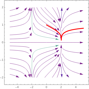
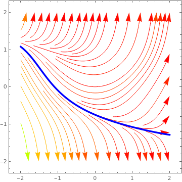
       Polynomial approximation (in red) and the actual solution (in blue).            Mathematica code


Taylor Series or Differential Transform Algorithm


The Taylor series method introduces the solution by an infinite series \( y(x) = \sum_{n\ge 0} c_n \left( x - x_0 \right)^n . \) The coefficients \( c_n = \frac{y^{(n)} (x_0 )}{n!} \) are expressed through the derivatives of the unknown function evaluated at the center that are in turn are determined recursively from the given initial value problem. The initial term follows from the initial condition c0 = y0. The first coefficient can also be found easily:

\[ c_1 = y' \left( x_0 \right) = f\left( x_0 , y_0 \right) . \]
Evaluation of the next coefficients requires differentiation
\[ c_2 = \frac{1}{2}\,y'' \left( x_0 \right) = \left. \frac{1}{2}\, \frac{{\text d}}{{\text d} x} \,f(x, y(x)) \right\vert_{x= x_0 , y= y_0} = \left.\frac{1}{2}\, \frac{\partial f}{\partial x} \right\vert_{x= x_0 , y= y_0} + \left.\frac{1}{2}\, \frac{\partial f}{\partial y} \right\vert_{x= x_0 , y= y_0} \, f(x_0 ,y_0 ) . \]
In general, we have
\[ c_n = \frac{1}{n!}\, y^{(n)} \left( x_0 \right) = \left. \frac{1}{n!}\, \frac{{\text d}^{n-1}}{{\text d} x^{n-1}} \,f(x, y(x)) \right\vert_{x= x_0 , y= y_0} , \qquad n=2,3,\ldots . \]
Practical implementation of this formula may be a challengeable problem even for a simple slope function such as a polynomial because it requires application of the chain rule. It becomes intractable in the general case because the number of terms grows exponential (see Faà di Bruno's formula). Therefore, this algorithm is used mostly to find a polynomial approximation by utilizing a computer algebra system, such as Mathematica that can help a lot with manipulations and simplifications, at least for first few terms.


Frobenius method


Although the method of solving linear diffeential equations with regular singular points was developed by L. Fuchs in 1866, G. Frobenius presented its simplification six years later. It is a custom to name it after the latter author. The Frobenius method is mostly effectively applicable in linear differential equations and some in limited classes of nonlinear equations for which the slope functions admits a power series expansion. For example when slope function contains a square or reciprocal of the unknown function. To demonstrate an application of the Frobenius method, we consider a simple initial value problem
\[ y' = y^2 , \qquad y(0) =1, \]
for which the explicit solution is known: y(x) = (1-x)-1. Substituting the power series \( y(x) = 1 + \sum_{n\ge 1} c_n x^n \) into the given differential equation and using the convolution formula, we obtain
\[ \sum_{n\ge 0} c_{n+1} \left( n+1 \right) x^n = \sum_{n\ge 0} \sum_{k=0}^n c_{n-k} c_k x^n . \]
Equating coefficients of like powers of x, we get a full history recurrence for determination of coefficients:
\[ c_{n+1} \left( n+1 \right) = \sum_{k=0}^n c_{n-k} c_k , \quad c_0 = 1, \qquad n=0,1,2,\ldots . \]


In all problems, y' denotes the derivative of function y(x) with respect to independent variable x and \( \dot{y} = {\text d} y/{\text d}t \) denotes the derivative with respect to time variable.
  1. Using ADM, solve the initial value problem: \( \left( 1 - xy \right) y' = y^2 , \qquad y(0) =1, \qquad (xy \ne 1) . \)
  2. Using ADM, solve the initial value problem: \( \left( x - y \right) y' = y , \qquad y(0) =1 , \qquad (y \ne x) . \)


  1. Dettman, J.W., Power Series Solutions of Ordinary Differential Equations, The American Mathematical Monthly, 1967, Vol. 74, No. 3, pp. 428--430.
  2. Fu, W.B., A comparison of numerical and analytical methods for the solution of a Riccati equation, International Journal of Mathematical Education in Science and Technology, `989, Vol. 20, No. 3, pp. 421--327.
  3. Grigorieva, E., Methods of Solving Sequence and Series Problems, Birkhäuser; 1st ed. 2016.
  4. Liao, S. and Tan, Y., A general approach to obtain series solutions of nonlinear differential equations, Studies in Applied Mathematics, 119(4, pp. 297--354.


Return to Mathematica page
Return to the main page (APMA0330)
Return to the Part 1 (Plotting)
Return to the Part 2 (First Order ODEs)
Return to the Part 3 (Numerical Methods)
Return to the Part 4 (Second and Higher Order ODEs)
Return to the Part 5 (Series and Recurrences)
Return to the Part 6 (Laplace Transform)
Return to the Part 7 (Boundary Value Problems)