Return to computing page for the second course APMA0340
Return to computing page for the fourth course APMA0360
Return to Mathematica tutorial for the first course APMA0330
Return to Mathematica tutorial for the second course APMA0340
Return to Mathematica tutorial for the fourth course APMA0360
Return to the main page for the course APMA0330
Return to the main page for the course APMA0340
Return to the main page for the course APMA0360
Return to Part I of the course APMA0330
Glossary
Preface
This section is devoted to aspects of qualitative analysis of first order differential equations in normal form. Other properties of the solution such as bounds, asymptotic expansions, stability, periodicity, etc., without explicitly solving the equation, will be explored later.
Qualitative Analysis
For a differential equation
When we model a practical phenomena, a physical system in perfect balance may be difficult to achieve(a coin standing on the edge) or easy to maintain (when you part your car). So behavior of a system can be hard to predict except some simple cases when we know the answer (oscillating pendulum). When a solution of the differential equation approaches a perfect balance, we say that it is coming to an equilibrium position. In this section, we discuss such behavior mostly for autonomous differential equations.
- If the derivative of the slope function at the critical point is negative, f(y*) < 0, then the equilibrium solution is asymptotically stable.
- If the derivative of the slope function at the critical point is positive, f(y*) > 0, then the equilibrium solution is unstable.
- If the derivative of the slope function at the critical point is zero, f(y*) = 0, then this test is inconclusive and the behavior of the solutions depends on the nonlinear terms.
Example: Consider the autonomous differential equation: \( y'= y^2 \) subject \( y(t_0) = y_0 = 2. \) Separating the variables, we get
The above conclusion becomes obvious for our particular case: t0 = 0 and y0 = 2. So, a continuous solution also exists on the interval \( (-\infty , 1/2) . \) If we change initial condition \( y(0) =-1 , \) the explicit solution becomes
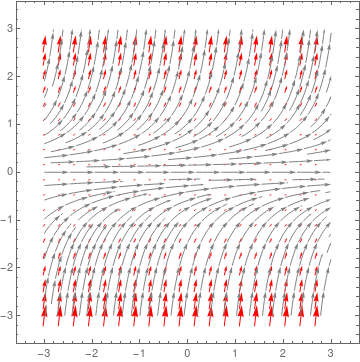
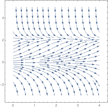
Upon plotting its direction field, we see that y = 0 is so called semi stable equilibrium solution because solutions started in negative semi-line approach y = 0 while solutions having positive initial conditions depart from the equilibrium solution.
|
StreamPlot[{1, y^2}, {x, -3, 3}, {y, -3, 3},
PerformanceGoal -> "Quality", StreamPoints -> Fine,
StreamStyle -> Gray, VectorPoints -> 20,
VectorStyle -> {Arrowheads[4], Red}]
|
| Phase portrait for y' = y² | Mathematica code |
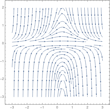
Example: Consider the not autonomous differential equation: \( y'= \left( 1- 3t \right) y^2 \) subject \( y(t_0) = y_0 = 2. \) Separating the variables, we get
|
StreamPlot[{1, (1 - 3*t)*y^2}, {t, -3, 3}, {y, -3, 3},
StreamScale -> 0.15]
Solve[-1/y == t-3/2*t^2 -1/y0 -t0 +3/2*t0^2, y]
{{y -> (2 y0)/(2 - 2 t y0 + 3 t^2 y0 + 2 t0 y0 - 3 t0^2 y0)}}
|
| Phase portrait for y' = (1-3t)y² | Mathematica code |
Example: Consider the autonomous differential equation
we conclude that y = 1 is unstable critical point and y = -1 is asymptotically stable equilibrium solution. However, y = -2 behaves differently from either of these two. Solutions that start below it move towards y = -2 while solutions that start above y = -2 move away as t increases. In cases where solutions on one side of an equilibrium solution move towards the equilibrium solution and on the other side of the equilibrium solution move away from it we call the equilibrium solution semi-stable. So y = -2 is a semi-stable equilibrium solution. ■
For the graphical analysis, we plot f(y) as a function of y. The points equilibria are the points of intersection of the graph f(y) with the horizontal axis. To determine stability, we check how solutions behave in a neighborhood of each point equilibrium. Plotting a direction field or phase portrait would be helpful.
The analytical analysis is based on linearization of the slope function about the equilibrium. The linearization of f(y) about the equilibrium y* is
Some applications in population modeling
In the very simplest and not realistic model, the growth rate r is assumed to be independent of the population size P and time t. Then its solution exhibits the Malthusian exponential growth law
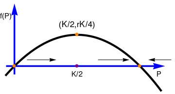
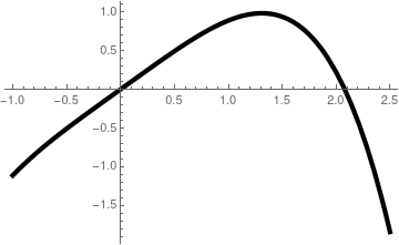
In a more realistic scenario, the growth rate will depend upon the size of the population as well as external environmental factors, including seasonable impact. For example, in the presence of limited resources, large population will have insufficient resources to increase. In other words, the growth rate r(P) > 0 when P < K, while r(P) < 0 when P > K, where the carrying capacity (or saturation level) K > 0 depends upon the resource availability. The simplest class of functions that satisfies these two inequalities are of the form
|
pp = Plot[P*(1-P/3), {P,-0.2,3.5}, PlotStyle->{Thickness[0.012], Black}, Axes->False]
axes1 = Graphics[{Blue, Thickness[0.01], Arrowheads[0.07], Arrow[{{-0.2,0},{3.6,0}}]}] axes2 = Graphics[{Blue, Thickness[0.01], Arrowheads[0.07], Arrow[{{0,-0.2},{0,1.5}}]}] p0 = Graphics[{PointSize[Large], Orange, Point[{0,0}]}] p3 = Graphics[{PointSize[Large], Orange, Point[{3,0}]}] p = Graphics[{PointSize[Large], Orange, Point[{3/2,3/4}]}] p2 = Graphics[{PointSize[Large], Purple, Point[{3/2,0}]}] ar1 = Graphics[Arrow[{{0.3,0.15},{1,0.15}}]] ar2 = Graphics[Arrow[{{2.0,0.15},{2.75,0.15}}]] ar3 = Graphics[Arrow[{{3.75,0.15},{3.2,0.15}}]] txt1 = Graphics[Text[Style["K/2", FontSize -> 14, Black], {3/2, -0.2}]] txt2 = Graphics[Text[Style["(K/2,rK/4)", FontSize -> 14, Black], {3/2, 1}]] txt3 = Graphics[Text[Style["f(P)", FontSize -> 14, Black], {-0.2, 1.2}]] txt4 = Graphics[Text[Style["P", FontSize -> 14, Black], {3.46, -0.2}]] Show[axes1,axes2,pp,p0,p,p2,p3,ar1,ar2,ar3,txt1,txt2,txt3,txt4] |
| Graph of f(P) | Mathematica code |
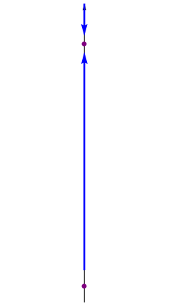
In this context the P-axis is often called the phase line, and it is reproduced in is in its more customary vertical orientation in the figure. The dots at P = 0 and P = K are the critical points, or stationary solutions. The arrows again indicate that P is increasing whenever 0 < P < K and that P is decreasing whenever P > K. Note that is P is near zero or K, then the slope f(P) is near zero, so the solution curves are relatively flat. They become steeper as the value of P leaves the neighborhood of zero or K.
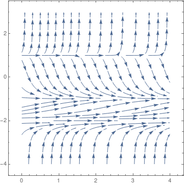
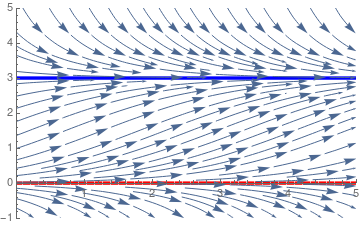
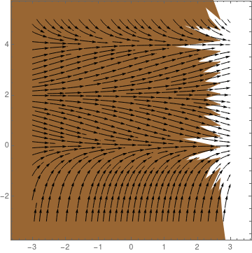
Then we plot the direction field using Mathematica command
StreamPlot:
|
|
a = Plot[0, {t, 0, 4}, PlotStyle -> {Thickness[0.01], Dashed, Red},
PlotRange -> {{0, 4}, {-1, 5}}]
b = Plot[3, {t, 0, 4}, PlotStyle -> {Thickness[0.01], Blue}, PlotRange -> {{0, 4}, {-1, 5}}] sp = StreamPlot[{1, P*(1 - P/3)}, {t, 0, 4}, {P, -1, 5}, StreamScale -> 0.12] Show[a, b, sp] a1 = Graphics[Arrow[{{0,-0.2}, {0,3.55}}]] a2 = Graphics[{Blue, Thickness[0.01], Arrowheads[0.07], Arrow[{{0,0.2}, {0,2.9}}]] a3 = Graphics[{Blue, Thickness[0.01], Arrowheads[0.07], Arrow[{{0,3.5}, {0,3.1}}]] p21 = Graphics[{PointSize[Large], Purple, Point[{0,3}]}] p22 = Graphics[{PointSize[Large], Purple, Point[{0,0}]}] Show[a1,a2,a3,p21,p22] |
| Phase portrait for the logistic equation | Mathematica code |
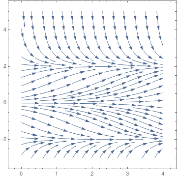
If we modify the logistic equation as
|
|
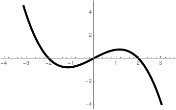
| Phase portrait for the modified logistic equation | Graph of slope function rP(1 - P²/K) |
we see that qualitatively the solutions behave in the same manner as in the logistic equation, at least in the first quadrant. Of course, there are three equilibrium solutions, but negative critical point P = -K does not matter for population model. Another model \( \dot{P} = r\,P \left( 1 - P^3 /K \right) \) has similar properties.
|
|
| Phase portrait for the modified logistic equation | Graph of slope function rP(1 - P³/K) |
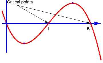
Example: The classical logistic threshold model may need to be modified so that unbounded growth does not occur when the population exceeds the threshold T. The simplest way to do this is to introduce another factor that will have the effect of making the velocity negative when the size of population becomes very large. Hence, we consider the model
p2 = Graphics[{PointSize[Large], Purple, Point[{3.1547005383787914, 0.38490017945975047}]}]
FindMinimum[-P*(1 - P/2)*(1 - P/4), {P, 1}]
pk = Graphics[{PointSize[Large], Purple, Point[{4, 0}]}]
pt = Graphics[{PointSize[Large], Purple, Point[{2, 0}]}]
p1 = Graphics[{PointSize[Large], Purple, Point[{0.8452994615144672, -0.3849001794597504}]}]
Show[slope, axes1, axes2, p1, p2, pk, pt]
|
|
| Phase portrait for the threshold logistic equation | Graph of slope function -rP(1 - P/K)(1 - P/T) |
Andrewartha and Birch (1954) pointed out the ecological importance of spatial structure to the maintenance of populations based on studies of insect populations. They observed that although local patches become frequently extinct, migrants from other patches subsequently recolonize extinct patches, thus allowing the population to persist globally.

In 1969, Richard Levins introduced the concept of metapopulations. This was a very influential paper that is highly cited even today. Richard Levins was of Ukrainian Jewish heritage and was born in Brooklyn, New York. Richard "Dick" Levins (1930--2016) was an extropical farmer turned ecologist, a population geneticist, biomathematician, mathematical ecologist, and philosopher of science who had researched diversity in human populations. Until his death, Levins was a university professor at the Harvard T.H. Chan School of Public Health and a long-time political activist. He was best known for his work on evolution and complexity in changing environments and on metapopulations. A metapopulation is a collection of subpopulations. Each subpopulation occupies a patch, and different patches are linked via migration of individuals between patches. Subpopulations may go extinct, thus leaving a patch vacant. Vacant patches may be recolonized by migrants from other subpopulations. This was a major theoretical advance: The metapopulation concept provided a theoretical framework for studying spatially structured populations, such as those studied by Andrewartha and Birch.
Levins' writing and speaking is extremely condensed. He was known throughout his lengthy career for his ability to make connections between seemingly disparate topics such as biology and political theory. This, combined with his Marxism, has made his analyses less well-known than those of some other ecologists and evolutionists who were adept at popularization. His research had the goal of making the obscure obvious by finding ways to visualize complex phenomena. Recent work examined the variability of health outcomes as an indicator of vulnerability to multiple non-specific stresses in human communities. One story of his Chicago years is that, in order to understand his lectures, his graduate students each needed to attend Levins' courses three times: the first time to acclimate themselves to the speed of his delivery and the difficulty of his mathematics; the second to get the basic ideas down; and the third to pick up his subtleties and profundities.
In Levins model, we keep track of the fraction of patches that is occupied by subpopulations. Subpopulations go extinct at a constant rate and we can set the time scale so that the rate is equal to 1. Vacant patches can be colonized at a rate that is proportional to the fraction of occupied patches; the constant of proportionality is denoted by k. If we call p(t) the proportion of occupied patches at time t, then writing \( p= p(t) , \) we find
To find equilibria, we set \( f(p) = k\,p \left( 1-p \right) -p \) and solve the equation f(p) = 0 for p:
We see that when 0 < k < 1, there is only one biologically relevant equilibrium, namely the trivial equilibrium p* = 0, which is locally stable. When k > 1, the trivial equilibrium becomes unstable, and a second equilibrium appears, \( p^{\ast} = 1- 1/k , \) which is locally stable.
a = Plot[g[x], {x, 0, 2}, PlotStyle -> {Thick, Black}]
b = Plot[0, {x, 1, 2}, PlotStyle -> {Dashed, Thick, Blue}]
Show[a, b]
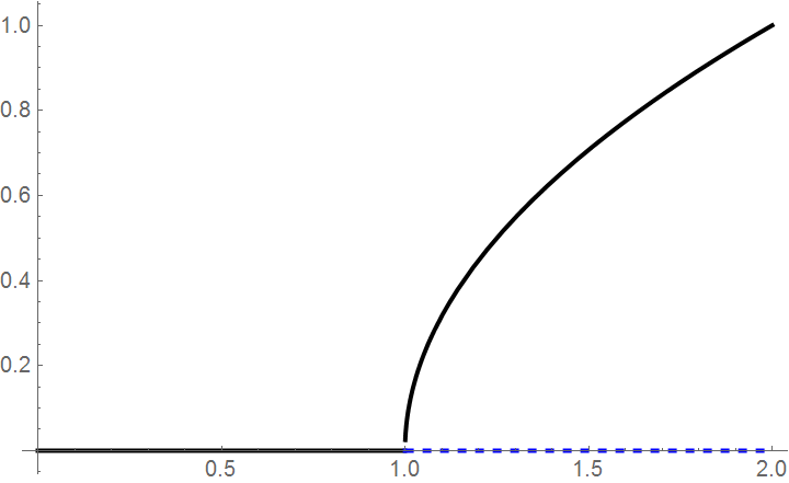
If we graph the equilibria as a function of the parameter k, we see that there is a qualitative change in behavior at k = 1. We call this a critical value k* =1 because for k < 1, the behavior is qualitatively different from the behavior when k > 1: the stability of the trivial equilibrium changes at k* =1 and a new and nontrivial equilibrium emerges. We will discuss this phenomenon in bifurcation section.
Return to Mathematica page
Return to the main page (APMA0330)
Return to the Part 1 (Plotting)
Return to the Part 2 (First Order ODEs)
Return to the Part 3 (Numerical Methods)
Return to the Part 4 (Second and Higher Order ODEs)
Return to the Part 5 (Series and Recurrences)
Return to the Part 6 (Laplace Transform) )
Return to the Part 7 (Boundary Value Problems)