Return to computing page for the second course APMA0340
Return to Mathematica tutorial for the second course APMA0340
Return to the main page for the course APMA0330
Return to the main page for the course APMA0340
Return to Part I of the course APMA0330
Glossary
Polar Plots
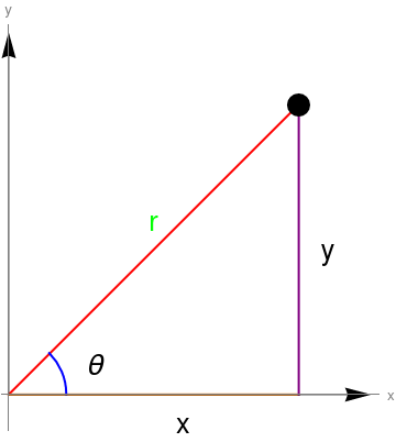
We use polar coordinates as an alternative way to describe points in the plane. In polar coordinates, we describe points via their angle (called argument or polar angle) with the positive x-axis measured in counterclockwise direction, and the distance from the origin (called radial distance). See figure below.
liner = Graphics[{Red, Thick, Line[{{0, 0}, {1, 1}}]}];
r = Graphics[Text[Style["r", Large, Green], {0.5, 0.6}]];
linex = Graphics[{Orange, Thick, Line[{{0, 0}, {1, 0}}]}];
x = Graphics[Text[Style["x", Large, Black], {0.6, -0.1}]];
y = Graphics[Text[Style["y", Large, Black], {1.1, 0.5}]];
liney = Graphics[{Purple, Thick, Line[{{1, 0}, {1, 1}}]}];
theta = Graphics[Text[Style["\[Theta]", Large, Black], {0.3, 0.1}]];
arc = Graphics[{Blue, Thick, Circle[{0, 0}, 0.2, {0, Pi/4}]}];
arrowx = Graphics[{Arrowheads[0.07], Arrow[{{0, 0}, {1.25, 0}}]}];
arrowy = Graphics[{Arrowheads[0.07], Arrow[{{0, 0}, {0, 1.25}}]}];
Show[{liner, r, linex, x, liney, y, arc, theta, point, arrowx, arrowy}, Ticks -> None, Axes -> True, AxesStyle -> Gray, AxesLabel -> {Style["x", Medium, Gray], Style["y", Medium, Gray]}]
Some other graphs:
Cycloid
The Parametrization
Manipulate[
ParametricPlot[
cycloid[a, b][t] // Evaluate, {t, -\[Pi]/2, 5*\[Pi]/2}], {a, 1, 5}, {b, 1, 5}]
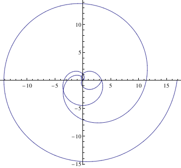
PolarPlot[Cycloid[1.5,theta],{theta, 0, 4*Pi}]
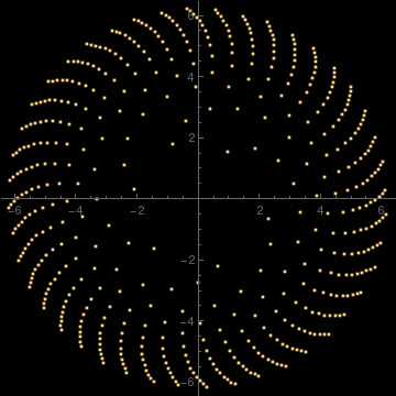
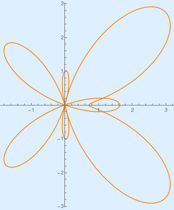
PolarPlot[{Exp[Cos[x]] - 2*Cos[4*x]}, {x, 0, 2*Pi}, PlotStyle -> {Orange}, Background -> LightBlue]
x = r*Cos[\[Theta]]; y = r*Sin[\[Theta]];
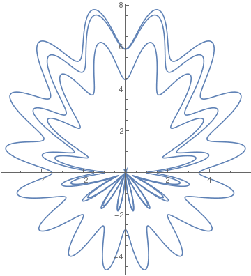
PolarPlot[r, {\[Theta], 0, 24 Pi}, Axes -> True, PlotRange -> {{-4, 4}, {-4, 4}}, Frame -> True, PlotPoints -> 1500, AspectRatio -> Automatic]
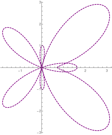
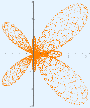
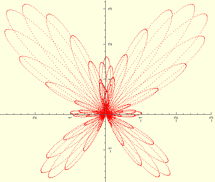
Butterfly curve. |
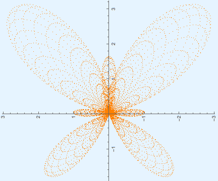
Butterfly curve with background. |
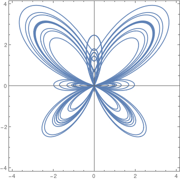
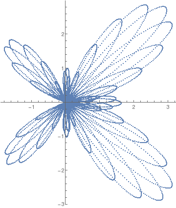
Rotated butterfly curve. |
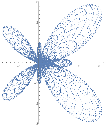
butterfly[99999998][0.0006]
butterfly[\[Lambda]_][h_, o___] := ListPolarPlot[ Table[{\[Theta], (Exp[Cos[\[Theta]]] - 2 Cos[4 \[Theta]])*(Sin[\[Lambda] \[Theta]]^4)}, {\[Theta], 0, 2 Pi, h}], o, PlotRange -> All, PlotStyle -> {PointSize[Tiny], Orange}, Background -> Lighter[LightBlue, 0.25]]
Rotate[%, 90 Degree]
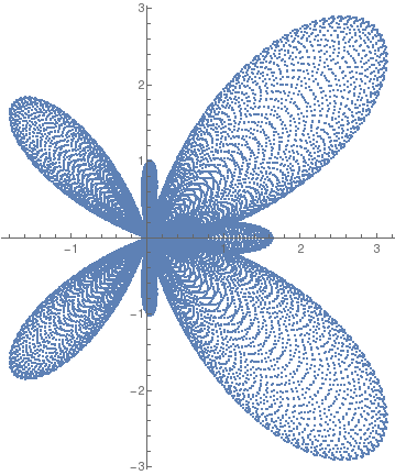
Butterfly curve. |
Butterfly curve on background. |
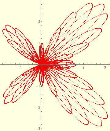
Rotated butterfly curve. |
butterfly[99999998][0.00065]
Rotate[%, 90 Degree]
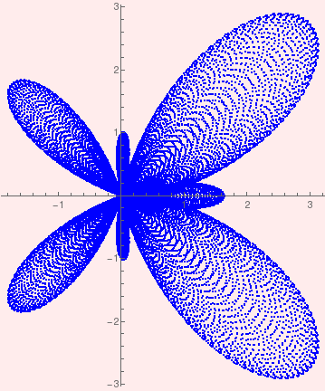
Butterfly curve with step size 0.00065. |
Butterfly curve with step size 0.00065 on background. |
Rotated butterfly curve curve with step size 0.00065. |
butterfly[\[Lambda]_][h_, o___] := ListPolarPlot[ Table[{\[Theta], (Exp[Cos[\[Theta]]] - 2 Cos[4 \[Theta]])*(Sin[\[Lambda] \[Theta]]^4)}, {\[Theta], 0, 2 Pi, h}], o, PlotRange -> All, PlotStyle -> {PointSize[Tiny], Blue}, Background -> LightPink]
butterfly[99999998][0.000169]
Rotate[%, 90 Degree]
Butterfly curve with step size 0.000169. |
Butterfly curve with step size 0.000169 on background. |
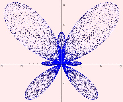
Rotated butterfly curve curve with step size 0.000169. |
- Geum, Y.H. and Kim, Y.I., On the analysis and construction of the butterfly curve using Mathematica, International Journal of Mathematical Education in Science & Technology, 2008, Vol. 39, Issue 5, pp. 670--678.
- Fay. T., The Butterfly curve, The American mathematical Monthly, 1989, Vol. 96, No 5, pp. 142--143.
- Fay. T., A study in step size, Mathematics magazine, 1997, Vol. 70, No. 2, pp. 116--117.
Return to Mathematica page
Return to the main page (APMA0330)
Return to the Part 1 (Plotting)
Return to the Part 2 (First Order ODEs)
Return to the Part 3 (Numerical Methods)
Return to the Part 4 (Second and Higher Order ODEs)
Return to the Part 5 (Series and Recurrences)
Return to the Part 6 (Laplace Transform)
Return to the Part 7 (Boundary Value Problems)