Preface
This is a tutorial made solely for the purpose of education and it was designed for students taking Applied Math 0330. It is primarily for students who have very little experience or have never used Mathematica before and would like to learn more of the basics for this computer algebra system. As a friendly reminder, don't forget to clear variables in use and/or the kernel.
Finally, the commands in this tutorial are all written in bold black font, while Mathematica output is in normal font. This means that you can copy and paste all commands into Mathematica, change the parameters and run them. You, as the user, are free to use the scripts for your needs to learn the Mathematica program, and have the right to distribute this tutorial and refer to this tutorial as long as this tutorial is accredited appropriately.
Return to computing page for the second course APMA0340
Return to Mathematica tutorial for the second course APMA0340
Return to Mathematica tutorial for the first course APMA0330
Return to the main page for the course APMA0340
Return to the main page for the course APMA0330
Return to Part III of the course APMA0330
Numerical Solutions
Although sometimes Mathematica is able to solve a differential equation, in practice we tend to rely on numerical methods to solve differential equations. Most differential equations that are found in actual practice are much too complicated to express a solution using elementary or special functions. Usually, we want to obtain a solution in implicit form, but unfortunately this only happens occasionally. It is important to note that because a differential equation does not have an explicit or implicit solution does not necessarily mean that the solution does not exist.
Since the kernel of a differential operator usually contains a space of functions, we do not expect to obtain a general solution that includes arbitrary constants. Instead, we knock out one solution by considering the initial value problem (IVP for short)
Example: Consider the initial value problem \( y' = \sin \left( x^2 \right) , \quad y(0) =0 . \) We try to find its solution using the standard Mathemaica command DSolve:
Now we solve the same problem numercally using NDSolve.

This indicates that y(6.5) approximately equal to 0.639918. We can improve accuracy by choosing the option PrecisionGoal
There are two main approaches to finding a numerical value for the solution to the initial value problem \( y' = f(x,y), \quad y( x_0 )= y_0 . \) Its solution can be obtained using either DSolve (for solutions represented using known functions, if it is possible) or NDSolve (for numerical solutions). The first one is based on definition of the slope function f(x,y) as an expression. The second one (which is recommended) is to define the slope as a function. To see how it works, let us consider an example.
Example: : Consider the slope function f(x,y) = 1/(3*x - 2*y + 1). Then we find a numerical value treating f(x,y) as an expression.
Now we use the function DSolve to find the explicit solution:
Solve::ifun: Inverse functions are being used by
Solve, so some solutions may not be found; use
Reduce for complete solution information. >>We present two other options to find a numerical value of a solution to the initial value problem using NDSolve.
y[x] /. sol /. x -> 3
http://library.wolfram.com/infocenter/Books/8503/AdvancedNumericalDifferentialEquationSolvingInMathematicaPart1.pdf
As we see applications of NDSolve
are very straightforward --- use the solution "interpolating function" as
a regular function. When plotting the solution, Mathematica recommends to use the Evaluation. We give some examples.
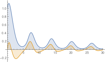
Example: First, we solve a first-order ordinary differential equation, which gives you decaying oscillations:
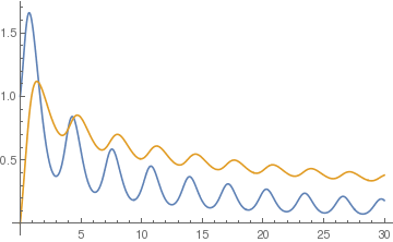
sol4 = NDSolve[{z'[x]== -z[x]+First[y[x]/5 + y'[x] /. sol3], z[0] == 0}, z, {x, 0, 30}];
Plot[{Evaluate[y[x] /. sol3], Evaluate[z[x] /. sol4]}, {x, 0, 30}, PlotRange -> All, Filling -> 0]
Return to Mathematica page
Return to the main page (APMA0330)
Return to the Part 1 (Plotting)
Return to the Part 2 (First Order ODEs)
Return to the Part 3 (Numerical Methods)
Return to the Part 4 (Second and Higher Order ODEs)
Return to the Part 5 (Series and Recurrences)
Return to the Part 6 (Laplace Transform)
Return to the Part 7 (Boundary Value Problems)