Preface
This section is devoted to a special modification of the Euler numerical rule, known as the Heun method.
Return to computing page for the second course APMA0340
Return to Mathematica tutorial for the first course APMA0330
Return to Mathematica tutorial for the second course APMA0340
Return to the main page for the course APMA0330
Return to the main page for the course APMA0340
Return to Part III of the course APMA0330
Glossary
Heun's Methods
According to the following definition, Heun's method is an explicit one-step method.
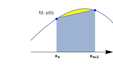
Trapezoid Rule
Suppose that we want to solve the initial value problem for the first order differential equation
 |
curve = Plot[x - Exp[x - 0.05] + 1.5, {x, -1.0, 0.7},
PlotStyle -> Thick, Axes -> False,
Epilog -> {Blue, PointSize@Large,
Point[{{-0.5, 0.42}, {0.25, 0.53}}]},
PlotRange -> {{-1.6, 0.6}, {-0.22, 0.66}}];
line = Plot[{0.43 + 0.44*0.5/3 + 0.44*x/3}, {x, -0.5, 0.25}, PlotRange -> {{0, 0.6}}, Filling -> Bottom, FillingStyle -> Opacity[0.6]]; curve2 = Plot[{x - Exp[x - 0.05] + 1.5, 0.43 + 0.44*0.5/3 + 0.44*x/3}, {x, -0.5, 0.25}, PlotStyle -> Thick, Axes -> False, PlotRange -> {{-1.6, 0.6}, {0.0, 0.66}}, Filling -> {1 -> {2}}, FillingStyle -> Yellow]; ar1 = Graphics[{Black, Arrowheads[0.07], Arrow[{{-1.0, 0.0}, {0.6, 0.0}}]}]; t1 = Graphics[ Text[Style["f(t, y(t))", FontSize -> 12], {-0.7, 0.5}]]; xn = Graphics[ Text[Style[Subscript["x", "n"], FontSize -> 12, FontColor -> Black, Bold], {-0.48, -0.05}]]; xn1 = Graphics[ Text[Style[Subscript["x", "n+1"], FontSize -> 12, FontColor -> Black, Bold], {0.24, -0.05}]]; Show[curve, curve2, line, ar1, t1, xn, xn1] |
To find its numerical solution, we pick up the uniform set of grid points \( x_n = x_0 + h\, n , \quad n=0,1,2,\ldots ; \) where the step size h is fixed for simplicity. As usual, we denote by yn approximate values of unknown function at mesh points \( y_n \approx \phi (x_n ) , \quad n=0,1,2,\ldots ; \) where ϕ is the actual solution of the given initial value problem (IVP for short).
The concept of the Trapezoidal Rule in numerical methods is similar to the trapezoidal rule of Riemann sums. The Trapezoid Rule is generally more accurate than the Euler approximations, and it calculates approximations by taking the sum of the function of the current and next term and multiplying it by half the value of h. Therefore the syntax will be as follows:
|
\begin{equation} \label{EqHeun.3}
y_{n+1} = y_n + \frac{h}{2} [ f( x_n , y_n ) + f( x_{n+1} , y_{n+1} ) ] , \qquad n=0,1,2,\ldots .
\end{equation}
|
|---|
A one-step explicit numerical method leads to a difference equation for discrete approximate values of the solution. As a rule, a discrete problem has much reacher properties than its continuous counterpart. Sometimes long term calculations may lead either to divergent process (referred to as instability) or to stable numerical solution---called the ghost solution---that has nothing in common with expected solution to the IVP, as was shown in Euler section. To avoid the instability and to prevent the appearance of ghost solutions for the long range calculation, many refined numerical procedures to integrate the ordinary differential equations have been proposed. In practical calculations, the central difference scheme is used when evaluations of slope function in intermediate points (as, for instance, required by Runge--Kutta methods) are not permitted. We mention two remedies to remove ghost solutions.
Consider the following mixed difference scheme parameterized by μ, 0 <μ<1, for the first order differential equation:Example: Consider the initial value problem for the linear equation
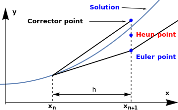
Heun's Formula / Improved Euler Method
The Improved Euler’s method, also known as Heun's formula or the average slope method, gives a more
accurate approximation than the Euler rule and gives an explicit formula for computing yn+1.
The basic idea is to correct some error of the original Euler's method. The syntax of the Improved Euler’s
method is similar to that of the trapezoid rule, but the y value of the function in terms of
yn+1 consists of the sum of the y value and the product of h and the function
in terms of xn and yn.
 |
curve = Plot[x^2 + 0.5, {x, 0.0, 1.7}, PlotStyle -> Thick,
Axes -> True, PlotRange -> {{0.0, 1.7}, {-0.22, 2.8}},
Epilog -> {Blue, PointSize@Large,
Point[{{1.25, 1.42}, {1.25, 1.83}, {1.25, 2.24}}]}];
line1 = Graphics[{Thickness[0.005], Line[{{0.5, 0.74}, {1.25, 1.42}, {2.0, 2.8}}], PlotStyle -> Black}]; line2 = Graphics[{Thickness[0.005], Line[{{0.5, 0.74}, {1.25, 2.24}}], PlotStyle -> Black}]; line2a = Graphics[{Dashed, Line[{{0.5, 0.74}, {0.5, 0.0}}]}]; line3a = Graphics[{Dashed, Line[{{1.25, 2.24}, {1.25, 0.0}}]}]; ar1 = Graphics[{Black, Arrowheads[{-0.04, 0.04}], Arrow[{{0.5, 0.22}, {1.25, 0.22}}]}]; h = Graphics[Text[Style["h", FontSize -> 12], {0.9, 0.35}]]; arx = Graphary = Graphics[{Black, Arrowheads[0.07], Arrow[{{0.05, -0.05}, {0.05, 2.60}}]}]; ary = Graphics[{Black, Arrowheads[0.07], Arrow[{{0.05, -0.05}, {0.05, 2.60}}]}]; x1 = Graphics[ Text[Style[Subscript["x", "n"], FontSize -> 12, FontColor -> Black, Bold], {0.5, -0.1}]]; x2 = Graphics[ Text[Style[Subscript["x", "n+1"], FontSize -> 12, FontColor -> Black, Bold], {1.25, -0.1}]]; x = Graphics[ Text[Style["x", FontSize -> 12, FontColor -> Black, Bold], {1.6, 0.25}]]; y = Graphics[ Text[Style["y", FontSize -> 12, FontColor -> Black, Bold], {0.14, 2.48}]]; euler = Graphics[ Text[Style["Euler point", FontSize -> 12, FontColor -> Blue, Bold], {1.49, 1.25}]]; heun = Graphics[ Text[Style["Heun point", FontSize -> 12, FontColor -> Red, Bold], {1.49, 1.85}]]; pr = Graphics[ Text[Style["Corrector point", FontSize -> 12, FontColor -> Black, Bold], {0.53, 2.22}]]; ar2 = Graphics[{Black, Arrowheads[0.02], Arrow[{{0.85, 2.22}, {1.2, 2.22}}]}]; s = Graphics[ Text[Style["Solution", FontSize -> 12, FontColor -> Blue, Bold], {1.4, 2.6}]]; ar3 = Graphics[{Black, Arrowheads[0.02], Arrow[{{1.16, 2.6}, {1.4, 2.56}}]}]; Show[curve, line1, line2, line2a, line3a, ar1, h, arx, ary, x1, x2, x, y, heun, euler, pr, ar2, s, ar3] |
|
\begin{equation} \label{EqHeun.5}
\begin{split}
p_{n+1} &= y_n + h\, f \left( x_n , y_n \right) , \\
y_{n+1} &= y_n + \frac{h}{2} [ f( x_n , y_n ) + f( x_{n+1} , p_{n+1} ) ], \quad n=0,1,2,\ldots . \end{split}
\end{equation}
|
|---|
nstep = 10;
f[x0_, y0_] := x0^2 + y0^2;
h = 0.1;
x0 = 0.0;
y0 = 1.0;
xy = Quiet@RecurrenceTable[
{
x[n + 1] == x[n] + h, x[0] == x0,
(* p[0] is just to conform to software's initalization *)
p[n + 1] == y[n] + h f[x[n], y[n]], p[0] == 0,
y[n + 1] == y[n] + h (f[x[n], y[n]] + f[x[n + 1], p[n + 1]])/2, y[0] == y0
},
{x, y}, {n, 0, nstep}, DependentVariables -> {x, y, p}]
|
Then we plot the discrete list {x,y}
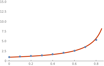
list=ListPlot[xy, PlotStyle -> PointSize[Large], PlotRange -> {0, 15}]
s = NDSolve[{y'[x] == x^2 + (y[x])^2, y[0] == 1}, y, {x, 0, 0.85}] plot = Plot[Evaluate[y[x] /. s[[1]]], {x, 0, 0.85}, PlotTheme -> "Web", PlotRange -> {0, 15}] Show[plot, list] |
|
|
Figure 3: Discrete Heun points along with true solution. |
Mathematica code |
Or using Do loop: Clear[y]
f[x_, y_] := x^2 + y^2
y[0] = 1;
h:=0.1;
Do[k1 = h f[h n, y[n]];
k2 = h f[h (n + 1), y[n] + k1];
y[n + 1] = y[n] + .5 (k1 + k2),
{n, 0, 9}]
y[10]
The main difference here is that instead of using y[n+1]=y[n]+h*f(x[n],y[n]), we use
Block[{ xold = x0,
yold = y0,
sollist = {{x0, y0}}, h
},
h = N[(xn - x0) / steps];
Do[ xnew = xold + h;
k1 = h * (f /. {x -> xold, y -> yold});
k2 = h * (f /. {x -> xold + h, y -> yold + k1});
ynew = yold + .5 * (k1 + k2);
sollist = Append[sollist, {xnew, ynew}];
xold = xnew;
yold = ynew,
{steps}
];
Return[sollist]
]
Instead of calculating intermediate values k1 and k2 , one can define ynew directly:
Block[{xold = x0, yold = y0, sollist = {{x0, y0}}, h},
h = N[(xn - x0)/steps];
Do[xnew = xold + h;
fold = f /. {x -> xold, y -> yold};
ynew =
yold + (h/2)*((fold) + f /. {x -> xold + h, y -> yold + h*fold});
sollist = Append[sollist, {xnew, ynew}];
xold = xnew;
yold = ynew, {steps}];
Return[sollist]]
The function heun is basically used in the same way as the function euler. Then to solve the
above problem, do the following:
Then read the answer off the table.
Another option:
h = 0.1
K = IntegerPart[1.2/h] (* if the value at x=1.2 needed *)
y[0] = 1 (* initial condition *)
Then implement Heun's rule:
y[n] + (h/2)*f[n*h, y[n]] + (h/2)*
f[h*(n + 1), y[n] + h*f[n*h, y[n]]], {n, 0, K}]
y[K]
One iteration step of the Heun method can be coded as follows
Module[{f, x0, y0, predict0, correct0, x1, h, corrector, predictor, y1},
{f, y0, x0, predict0, correct0, h} = args;
{f, y1, x1, predictor, corrector, h}
];
- list
- line
- plot
- table
https://www.wolfram.com/language/elementary-introduction/2nd-ed/34-associations.html
https://reference.wolfram.com/language/ref/Association.html
https://reference.wolfram.com/language/guide/Associations.html
We need often to have similar structure but no error issued if index is not available.
Association or <| |> addresses these issues and much more:
assoc[0]
In the following code, a return value variable called res
res=func[... ] ;
To figure out what is inside Association, use Keys:
Keys@res
res["plot”] outputs the plot
Module[{list, f, y0, x0, predict0, correct0, h, xy, tmp},
list = {};
{f, y0, x0, predict0, correct0, h} = args;
NestList[(AppendTo[list, {#, oneHeun[#]}]; oneHeun[#]) &, {f, y0, x0, predict0, correct0, h}, n];
xy = Table[{list[[i]][[1]][[3]], list[[i]][[1]][[2]]}, {i, 1, Length@list}];
<|
"list" -> list,
"poly line" -> xy,
"plot" ->
ListLinePlot[xy, PlotRange -> All, PlotTheme -> "Web", FrameLabel -> syms,
PlotLabel -> Row@{"Heun Solution to " <> syms[[2]] <> "'" <> "=", TraditionalForm@f[syms[[2]], syms[[1]]]}],
"table" -> (Dataset@Table[ tmp = Drop[list[[i]][[1]], 1];
<|
syms[[1]] -> tmp[[2]],
syms[[2]] -> tmp[[1]],
"predictor" -> tmp[[3]],
"corrector" -> tmp[[4]]
|>,
{i, 1, Length@list, 19}]),
"true solution" -> (
Block[{y, x, s},
y = ToExpression[syms[[2]]];
x = ToExpression[syms[[1]]];
s = NDSolve[{y'[x] == f[y[x], x], y[list[[1]][[1]][[3]]] == list[[1]][[1]][[2]]}, y, {x, list[[1]][[1]][[3]], n*h}];
Plot[ Evaluate[y[x00] /. s[[1]]], {x00, list[[1]][[1]][[3]], n*h}, PlotRange -> All]
]
)
|>
];
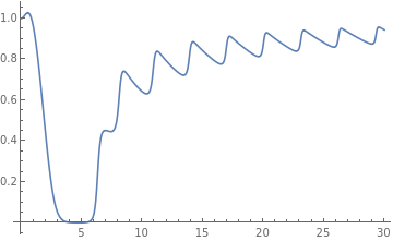
Example: Consider the initial value problem for the first order differential equation with oscillating slope function
f[y_, t_] := y*Cos[t + y];
h = 0.1; x0 = 0.0; y0 = 1;
predictor = y0 + h*f[y0, x0];
x1 = x0 + h;
corrector = y0 + h*(f[y0, x0] + f[predictor, x1])/2.0;
n = 300;
args = {f, y0, x0, corrector, predictor, h};
res = heunNETLIST[args, n, {"t", "y"}];
Keys@res
{"list", "poly line", "plot", "table"}
res["plot"]
| t | Heun solution | Predictor | NDSolve |
|---|---|---|---|
| 0.0 | 1 | 1.04835 | 1.0 |
| 1.9 | ??? | ??? | ??? |
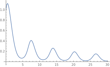
Example: Consider the initial value problem for the first order differential equation with oscillating slope function
Clear[f];
f[y_, t_] := Sin[t*y]*Cos[t + y];
h = 0.1; x0 = 0.0; y0 = 1;
predictor = y0 + h*f[y0, x0];
x1 = x0 + h;
corrector = y0 + h*(f[y0, x0] + f[predictor, x1])/2.0;
n = 300;
args = {f, y0, x0, corrector, predictor, h};
res = heunNETLIST[args, n, {"t", "y"}];
res["plot"]
| t | Heun solution | Predictor | NDSolve |
|---|---|---|---|
| 0.0 | 1 | 1.00226 | 1.0 |
| 1.9 | 0.500292 | 0.500263 | ??? |
Example: Consider the initial value problem for the linear equation
Example: Consider the initial value problem for the logistic equation
Example: Consider the initial value problem for the Riccati equation
heun routine, we get
Example: Consider the initial value problem \( y'= 1/(3x-2y+1),\quad y(0)=0 \)
First, we find its solution using Mathematica's command DSolve:
DSolve[{y'[x] == f[x, y[x]], y[0] == 0}, y[x], x]
To evaluate the exact solution at x=1.0, we type
y[x] /. a /. x -> 1.0
Then we use Heun's numerical method with step size h=0.1:
Do[k1 = h f[n*h, y[n]]; k2 = h f[h*(n + 1), y[n] + k1];
y[n + 1] = y[n] + 0.5*(k1 + k2), {n, 0, 9}]
y[10]
Now we demonstrate the use of while command:
i = 1
h=0.1;
Array[x, Nsteps];
Array[y, Nsteps];
While[i < Nsteps+1, x[i] = x[i - 1] + h; i++];
k=1
While[k < Nsteps,
y[k] = y[k - 1] + (h/2)*
Function[{u, v}, f[u, v] + f[u + h, v + h*f[u, v]]][x[k - 1], y[k - 1]];
k++];
Array[y, Nsteps] (* to see all Nsteps values *)
y[Nsteps] (* to see the last value *)
Example: Let us take a look at the initial value problem for the integro-differential equation
Numerical experiment with iterations
y[0] =50
Heun's method: To approximate the solution of the initial value problem \( y' = f(x,y), \ y(a ) = y_0 \) over [a,b] by computing
Make a computational experiment: in the improved Euler algorithm, using the corrector value as the next prediction, and
only after the second iteration use the trapezoid rule.
The ``improved'' predictor-corrector algorithm:
k_1 &= f(x_k , y_k ) ,
\\
k_2 &= f(x_{k+1} , y_k + h\,k_1 ) ,
\\
k_3 &= y_k + \frac{h}{2} \left( k_1 + k_2 \right) ,
\\
y_{k+1} &= y_k + \frac{h}{2} \left( k_1 + k_3 \right) ,
\end{align*} \]
Block[{xold = x0, yold = y0, sollist = {{x0, y0}}, h},
h = N[(xn - x0)/steps];
Do[xnew = xold + h;
k1 = f[xold, yold];
k2 = f[xold + h, yold + k1*h];
k3 = yold + .5*(k1 + k2)*h;
ynew = yold + .5*(k1 + f[xnew, k3])*h;
sollist = Append[sollist, {xnew, ynew}];
xold = xnew;
yold = ynew, {steps}];
Return[sollist]]
Then we apply this code to numerically solve the initial value problem \( y' = (1+x)\,\sqrt{y} , \quad y(0) =1 \) with step size h=0.1:
heunit[f, {x, 0, 2}, {y, 1}, 20]
Return to Mathematica page
Return to the main page (APMA0330)
Return to the Part 1 (Plotting)
Return to the Part 2 (First Order ODEs)
Return to the Part 3 (Numerical Methods)
Return to the Part 4 (Second and Higher Order ODEs)
Return to the Part 5 (Series and Recurrences)
Return to the Part 6 (Laplace Transform)
Return to the Part 7 (Boundary Value Pr