This secton is devoted to a special class of variable coefficients linear
differential equations. This remarkable class was discovered by Leonhard Euler
who showed that these differential equations could be solved explicitely via elementary functions.
Return to computing page for the first course APMA0330
Return to computing page for the second course APMA0340
Return to Mathematica tutorial for the first course APMA0330
Return to Mathematica tutorial for the second course APMA0340
Return to the main page for the course APMA0330
Return to the main page for the course APMA0340
Return to Part IV of the course APMA0330
An Euler equation (also known as the Euler-Cauchy equation, or equidimensional equation) is a
linear homogeneous ordinary differential equation with variable coefficients of the following form:
where the coefficients \( a_0 , a_1 , \ldots , a_n \) are constants and the driving function
f(x) is given. Since the leading term in the Euler equation is a multiple of xn, the origin
should be excluded from consideration. The Euler equation is usually considered on semi-infinite intervals either
\( (0, \infty ) \quad\mbox{or}\quad (-\infty , 0) . \) Let
be the linear differential operator corresponding to the Euler equation. We start with finding functions annihilated
by the Euler operator; in other words, we are going to determine the fundamental set of solutions for the homogeneous
equation \( L\left[ x, \texttt{D} \right] y = 0 \) on the positive semi-axis
\( (0, \infty ) . \)
There are known two methods to solve the homogeneous Euler equation. One is to try a power function \( y = x^m , \)
which leads to
Here \( \displaystyle m^{\underline{k}} = m(m-1) \cdots (m-k+1) \) is k-th falling factorial of number m.
Applying the above Euler operator to a trial solution xm, we obtain
where P(m) is an auxiliary polynomial of degree n (in accordance to the degree of the Euler operator).
If m is a root of the above algebraic equation, then \( y = x^m \) is a
solution of the n-th order Euler homogeneous equation. We postpone analyzing the fundamental set of solutions,
which depends on whether the roots of the auxiliary algebraic equation are real or complex and whether some of them
have multiplicities others than 1.
Because of the particularly simple equidimensional structure, the Euler equation can be replaced with an
equivalent constant coefficients differential equation, which can then be solved explicitly. Using change of independent variable
\( x = e^t , \quad t = \ln x ,\) it follows that
and so on. So we see that every derivative with respect to x, upon transformation to a new variable t, has
a multiple reciprocal to x; therefore, all these power multiples are canceled out and we obtain a constant
coefficient differential equation. We summarize our observation in the table:
Thus, \( y= x^m \) is a solution of the Euler equation if and only if m is a root of
the auxiliary polynomial
\[
P(m) = a\,m(m-1) + b\,m + c ,
\]
which simplifies to
\[
P(m) = a\,m^2 + \left( b-a \right) m + c .
\]
If P(m) has two distinct roots, either real or complex, we know how to solve the
equation. To recall briefly, if P(m) has two distinct real roots m1 and m2,
then \( x^{m_1} \quad\mbox{and}\quad x^{m_2} \) are two linearly independent solutions of
the Euler equation; hence, the general solution becomes
\[
y= C_1 x^{m_1} + C_2 x^{m_2} ,
\]
for some arbitrary constants C1 and C2.
If P(m) has two distinct complex roots \( m_1 \quad\mbox{and}\quad m_2 , \)
they must be complex conjugates, so we can write \( m_1 = \alpha + \beta {\bf j} \) and
\( m_2 = \alpha - \beta {\bf j} , \) where α and β are real numbers and j
is a unit vector in positive vertical direction on the complex plane, so \( {\bf j}^2 =-1 . \)
It's perhaps not so clear what a complex power of x means, but since x is assumed to be positive,
we have \( x = e^{\ln x} = e^t . \) If the complex power makes any kind of sense, we ought to have
Verifications of these equations we leave to Mathematica.
f[x_, a_] = x^a *(Cos[b*Log[x]] + I*Sin[b*Log[x]])
TrueQ[Simplify[D[f[x, a], x]] - (a + b*I)*f[x, a - 1] == 0]
True
We can also check that our two complex solutions \( y_1 = x^{\alpha + {\bf j}\,\beta} \) and
\( y_2 = x^{\alpha - {\bf j}\,\beta} \) are linearly independent by computing their Wronskian
where A1 and A2 are arbitrary complex numbers. Each complex number is an ordered pair
of two real numbers, so the above complex solution contains four arbitrary real constants. Since we are after a real-valued solution,
we have to exclude two of them and impose additional constraint: \( A_2 = \overline{A_1} , \) so they should be complex conjugate.
In this case, we reduce our general form of solution to the form
Finally, we consider the case when the auxiliary polynomial P(m) has one double root: \( P(m) = a\left( m- m_1 \right)^2 . \)
Then we have the only one solution expressed through a power function:
\( y_1 = x^{m_1} . \) So we we need to find a second
solution that is independent of y1. This can be done by the method of reduction of
order. To apply this method we look for a solution of the Bernoulli form
\( y = u(x)\,y_1 , \) where y1
is the solution we already know. Before plugging this in, we need to rewrite the
differential equation in the right form by expanding the auxiliary polynomial:
\( P(m) = a \left( m- m_1 \right)^2 = a\, m^2 - 2a\, m_1 m + a\,m_1^2 . \) Equating it to
\( P(m) = a\,m^2 + \left( b-a \right) m + c , \) we find
Finally, there is the case where P(m) has only one real root r
of multiplicity two. In this case, we get one solution \( y_1 = x^r \) of the
Euler equation and we need to find a second solution that is independent of y1.
This can be done by the method of reduction of
order. To apply this method we look for a solution of the form \( y = u(x)\,y_1 = u(x)\,x^r .\)
Before plugging this in, we need to rewrite the
differential equation in the right form.
We need to express coefficients in terms of the double root:
\[
\frac{{\text d}v}{v} = -\frac{{\text d}x}{x} \qquad\Longrightarrow \qquad \ln v = -\ln x + C = \ln x^{-1} +C = \ln C\,x^{-1} ,
\]
where C is a constant of integration. Therefore, we have
\[
v = C\, x^{-1} .
\]
We’re only looking for one u that works, so we can choose the value of C,
say C = 1. This gives us
\[
u' = v = x^{-1} \qquad\Longrightarrow \qquad u = \ln x + C .
\]
Again, we can set the constant of integration to 0 because we’re only looking for
one u that works. Plugging into our trial solution, \( y = u(x)\,y_1 = u(x)\,x^r ,\)
we conclude that the second solution of the Euler equation in the case of a double root r is
\( y = x^r \ln x , \quad x>0. \)
It’s pretty clear that these are independent solutions, so the general solution of the Euler equation in the
case of a double root r is
\[
y = v = C_1 x^r + C_2 x^r \ln x .
\]
Example:
Consider the homogeneous differential equation
\[
x^2 y'' + 7x \,y' -7\,y =0 .
\]
Guided by the theory, we only need to find two linearly independent solutions of the above equation. Substituting the trial solution
\( y = x^m , \) we obtain auxiliary algebraic equation
\[
m^2 + 6\, m - 7 =0 .
\]
Since it has two distinct real roots \( m = -7 \quad\mbox{and} \quad m =1 , \) we get the general solution
\[
y = C_1 x^{-7} + C_2 x .
\]
Example: Solve the homogeneous Euler equation
\[
4x^2 y'' +8x \,y' + y =0 .
\]
Upon substitution of the trial solution \( y = x^m , \) we obtain auxiliary algebraic equation
when \( m^2 -2m +5 =0 . \) From the quadratic formula we find that the roots are
\( m_1 = 1 + 2{\bf j} \) and \( m_2 = 1 - 2{\bf j} . \) With
the identifications α = 1 and β = 2, we find the general solution:
\[
y = x \left[ C_1 \cos (2\,\ln x) + C_2 \sin (2\,\ln x) \right] .
\]
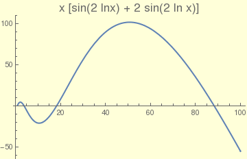
By applying the initial conditions \( y(1) =1, \ \ y'(1) =5 \) to the foregoing solution
and using \( \ln 1 =0 , \) we then find, in turn, that \( C_1 =1 \)
and \( C_2 =2 . \) Hence, the solution of the initial value problem is
\[
y = x \left[ \cos (2\,\ln x) + 2\, \sin (2\,\ln x) \right] .
\]
Substituting in the given differential equation and simplifying yields
\[
\ddot{y} -4\,\dot{y} + 3\,y = 3\,t .
\]
Since the last equation has constant coefficients, the characteristic polynomial corresponding to the homogeneous equation
is \( \lambda^2 -4\,\lambda + 3 = \left( \lambda -3 \right) \left( \lambda -1 \right) . \)
Since its nulls are λ =1 and &lambda: =3, the general solution in variable t of the corresponding homogeneous equation is
\[
y_h = C_1 e^t + C_2 e^{3t} ,
\]
with some constants C1 and C2.
Using method of undetermined coefficients, we seek a particular solution as a polynomial of first degree (similar to the
right-hand side function):
\[
y_p = a+ bt ,
\]
This assumption leads to b =1 and a = 4/3. Using \( y = y_h + y_p , \) we
get the general solution in variable t:
\[
y = y_h + y_p = C_1 e^t + C_2 e^{3t} + \frac{4}{3} + t .
\]
Now we return to the original variable x:
\[
y(x) = C_1 x + C_2 x^3 + \frac{4}{3} + \ln x .
\]
Example:
Solve the nonhomogeneous Euler equation for positive x:
\[
x^2 y'' -x\,y' + y = x^3 e^x .
\]
Since the given equation is nonhomogeneous, we first need to find the fundamental set of solutions for the associated homogeneous equation
\( x^2 y'' -x\,y' + y = 0 . \) Using a trial solution \( y = x^m , \)
we determine the auxiliary equation \( m(m-1) -m + 1=0 \) or
\( (m - 1)^2 =0 . \) In case of one double root, we obtain two linearly independent solutions
\( y_1 = x \quad\mbox{and}\quad y_2 = x\,\ln x . \) Then the general solution of the associated homogeneous equation becomes
\( y_h = C_1 y_1 + C_2 y_2 = C_1 x + C_2 x \,\ln x . \)
Now we are ready to attack our main nonhomogeneous equation. According to the variation of parameters, we seek a particular solution as a linear combination:
\[
y_p = A(x)\, y_1 + B(x) \, y_2 = A(x)\, x + B(x) \,x\, \ln x ,
\]
where derivatives of the unknown functions A(x) and B(x) are determined from the Lagrange system of algebraic equations
\begin{align*}
A' (x) \, x + B' (x) \,x\,\ln x &= 0,
\\
A' (x) + B' (x) \, \ln x + B' (x) &= x\, e^x .
\end{align*}
Solving this system is not hard to obtain
\[
\begin{split}
A' (x) &= -x\,e^x \, \ln x ,
\\
B' (x) &= x\, e^x ;
\end{split} \qquad\Longrightarrow \qquad \begin{split}
A (x) &= -\int x\,e^x \, \ln x \,{\text d}x = e^x - \mbox{Ei} (x) - e^x \left( x-1 \right) \ln x ,
\\
B' (x) &= \int x\, e^x \,{\text d}x = e^x \left( x-1 \right) ,
\end{split}
\]
where Ei(x) is the exponential integral, which has to be understood in terms of the Cauchy principal value due
to the singularity of the integrand at zero:
Example:
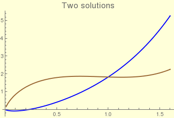
Suppose that we know the fundamental set of solutions \( y_1= x^3 \quad \mbox{and} \quad y_2 =x^{-1}\)
for the differential equation \( x^2 y'' -x\,y' -3y =0 . \)
If the right-hand side function is \( (x-3)^2 /x , \) we need to solve the nonhomogeneous equation
where \( W(x) \) is the Wronskian of \( y_1 , y_2 . \)
Now we determine the linear differential operator \( L[x, \texttt{D}] \) having
\( y_1 (x) \ \mbox{and} \ y_2 (x) \) as solutions of \( L[x, \texttt{D}]\, y=0. \)
has always one real null. Two other nulls could be either complex conjugate pair (recall that we consider only equations with real coefficients)
or two real numbers. Depending on these cases, the general solution is expressed as a linear combination through the
corresponding fundamental set of solutions. However, the pattern is clear. Therefore, we conclude this section
with two illustrative examples.
Example:
Consider a third order Euler equation
\[
x^3 y''' + x\,y' - y =0 .
\]
Plugging a trail solution \( y = x^m \) into the given equation, we obtain the auxiliary polynomial
where unknown functions should be determined from the Lagrange system of equations for their derivatives:
\begin{align*}
A' (x) \, x + B' (x) \,x^2 + C' (x) \, x^{-1} &= 0,
\\
A' (x) + B' (x) \, 2x - C' (x) \, x^{-2} &= 0,
\\
2\, B' (x) + 2\, C' (x) \, x^{-3} &= \ln x .
\end{align*}
We ask Mathematica to provide us a solution for the above system of algebraic equations, and it did not refuse:
Return to Mathematica page
Return to the main page (APMA0330)
Return to the Part 1 (Plotting)
Return to the Part 2 (First Order ODEs)
Return to the Part 3 (Numerical Methods)
Return to the Part 4 (Second and Higher Order ODEs)
Return to the Part 5 (Series and Recurrences)
Return to the Part 6 (Laplace Transform)
Return to the Part 7 (Boundary Value Problems)