A scalar Riccati differential equation is an equation of the form \( y' + p(x)\,y = g(x)\,y^{2} + f(x) , \quad \) where p, g, and f are given continuous on some finite interval real-valued functions, and g(g) ≠ 0.
The Riccati equation is used in different areas of physics, engineering, and mathematics such as quantum mechanics, thermodynamics, and control theory. However, most applications use vector Riccati differential equation with some matrices instead of mentioned above functions---the corresponding dynamic systems are discussed in the second course APMA0340.
There are numerous online video tutorials covering this subject, one of the best is at this link. They describe a sequence of steps that convert the Riccati equation to either a Bernoulli equation or a linear differential equation. These involve knowing in advance a particular solution, applying non-negative constraints judiciously to certain terms and then careful substitutions of identities obtained from the specific solution to reach the general solution.
This entire web page, including all Wolfram language code, is available for download at this link.
Return to computing page for the first course APMA0330
Return to computing page for the second course APMA0340
Return to Mathematica tutorial for the first course APMA0330
Return to Mathematica tutorial for the second course APMA0340
Return to Mathematica tutorial for the fourth course APMA0360
Return to the main page for the course APMA0330
Return to the main page for the course APMA0340
Return to the main page for the course APMA0360
Return to Part II of the course APMA0330
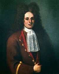
Jacopo Francesco Riccati (1676--1754) was an Venetian mathematician and jurist from Venice. In 1724, he considered the particular differential equation
\[
u' (x) = n\,x^{m+n-1} - x^{-n} u^2 (x) ,
\]
where m and n are real constants. Later, this equation was generalized to the first order non-linear equation, which now bears Riccati's name:
where p, g, and f are some real-valued given functions on finite interval [𝑎, b]. According to G.N. Watson, the designation of Eq.(1) as “Riccati’s equation” was made by d’Alembert in 1768 (Histoire de l'Académie royale des sciences et des Belles Lettres de Berlin, XIX, 1768; published 1770, page 242). Actually, differential equation (1) was known to mathematical community somewhat earlier, primarily to Daniel Bernoulli (1700--1782). In fact, Riccarti refused to dispute his priority of discovering equation (1), saying that he had no intention to challenge the Bernoulli family.
Jacopo Riccati was educated first at the Jesuit school for the nobility in Brescia, and in 1693 he entered the
University of Padua to study law. He received a doctorate in law in 1696. Encouraged by Stefano degli
Angeli to pursue mathematics, he studied mathematical analysis. Riccati received various academic offers,
but declined them in order to devote his full attention to the study of mathematical analysis on his own.
Peter the Great invited him to Russia as president of the St. Petersburg Academy of Sciences. He was also
invited to Vienna as an imperial councilor and was offered a professorship at the University of Padua.
He declined all these offers. He was often consulted by the Senate of Venice on the construction of canals and dikes along rivers.
When f(x) = 0, we get a Bernoulli equation. If g(x) = 0, the equation becomes a first order linear ordinary differential equation. Therefore, we exclude these trivial cases from our consideration. It is well known that solutions to the general Riccati equation are not available; therefore, it is desirable to simplify the Riccati equation by substitution. The first observation given below shows that the coefficient g(x) can always be dropped by considering it as 1 subject to g(x) ≠ 0.
Lemma 1:
Let y(x) be a solution of the Riccati equation y′ + p(x) y = g(x) y² + f(x) on some interval where g(x) ≠ 0.
Upon substitution y = u/g into this Riccati equation, the new dependent variable u becomes a solution of the following Riccati equation
\[
u' + \left( p - \frac{g'}{g} \right) u = u^2 + g\,f , \qquad g(x) \ne 0 .
\]
Substitution of y = u/g into the Riccatu equation yield
\[
\frac{1}{g}\, u' - \frac{g'}{g^2}\, u + \frac{p}{g}\, u = g \left( \frac{1}{g}\,u \right)^2 + f .
\]
Multiplying both sides of the latter, we obtain
\[
u' - \frac{g'}{g}\, u + p\, u = u^2 + g(x)\,f(x) .
\]
On the other hand, the linear term can be dropped by making the coefficient p(x) = 0. This can be achieved when g(x) ≠ 0 by substitution
\[
y = w\,\exp \left\{ \int p(x)\,{\text d} x \right\} .
\]
Under this substitution, the function w(x) satisfies
Therefore, every Riccati equation can be reduced to the equation in normal form (3) with coefficient B(x) = 1 of the square term. There are known many other transformations that reduce the Riccati equation to specific form (3); consult the text by Polyanin & Zaitsev.
Continuing to use Wolfram code to verify the above; we first define the functions p, g, f, and their derivatives as functions of x:
Define the new Riccati equation for w in normal form
wPrime = a[x] + w[x]^2;
Display the resulting expression for A (x) and the Riccati equation in normal form
TableForm[{a[x], wPrime}]
It is widely known that most differential equations do not have a solution expressed in closed form. This web page provides examples of those that may be solved in explicit form, often with techniques which may be thought of as "devices" or in more recent technology slang, "protips." These include knowing or assuming a single solution, as we are using here, or assuming certain relations between coefficients. Many transformations and substitutions lead to proper answers for specific differential equation types. Such devices may take liberties with strict rules of proof but are useful in the real world.
Because of the wide variety of these techniques, it is very difficult to present a comprehensive view of all the possible permutations that may arise. For this reason, the code results in this webpage may not strictly match the answer that a computer code delivers. This NOT to say that one of two different forms of the same answer is wrong, just that simplifications of one can produce an equally correct alternative form of the same answer. One way to reconcile different forms, and an excellent exercise for the student, is to assume fixed values for variables and insert those values into the two different forms. If the result of both produce the same numeric value you may be satisfied that the two forms describe the same (correct) answer.
Example 1:
We consider the Riccati equation
\[
y' + y = e^x y^2 + 4\,e^{-x} .
\tag{1.1}
\]
The substitution
\[
y = e^{-x} u \qquad \Longrightarrow \qquad u' = u^2 +4
\]
reduces this equation (1.1) to a separable equation
\[
\frac{{\text d}u}{u^2 + 4} = {\text d}x \qquad \Longrightarrow \qquad \int \frac{{\text d}u}{u^2 + 4} = \frac{1}{2}\,\arctan \left( \frac{u}{2} \right) = x + C .
\]
Integrate[1/(u^2 + 4), u]
1/2 ArcTan[u/2]
Hence, the general solution of the Riccati equation (1.1) becomes
\[
\arctan \left( \frac{e^x y}{2} \right) = 2x + C .
\]
■
End of Example 1
One of the strengths of the Riccati equation is that it is a unifying link between linear differential equations and non-linear equations.
As so, the Riccati equation has much in common with linear
equations; for example, it has no singular solution. Except special cases, the Riccati equation cannot
be solved analytically using elementary functions or quadratures, and the most common way to obtain its
solution is to represent it in series or apply a numerical solver. Moreover, the Riccati equation can be reduced to the second order
linear differential equation by Euler's substitution
Example 2:
We consider the Riccati equation
\[
y' + 3\,x^2 y(x) = x\, y^2 + \sinh x ,
\tag{2.1}
\]
where y′ = dy/dx is the derivative of unknown function y(x). Application of Euler's substitution \( \displaystyle \quad y = - u'/(x\,u) \ \) yields
\[
- \frac{u''}{x\,u} + \frac{u'}{x^2 u} + \frac{(u' )^2}{x\,u^2} - 3x\,\frac{u'}{u} = x \left( \frac{u'}{x\,u} \right)^2 + \sinh x .
\]
Canceling square terms, we simplify this equation as
\[
- \frac{u''}{x\,u} + \frac{u'}{x^2 u} - 3x\,\frac{u'}{u} = \sinh x
\]
or upon multiplication by x u, we get a linear equation
\[
- u'' + u' \left( \frac{1}{x} - 3x^2 \right) = x\,u\,\sinh x .
\tag{2.2}
\]
We can make another substitution
\[
w = \exp \left\{ - \int x\,y(x)\,{\text d} x \right\} .
\]
Now we calculate the expression with some coefficients 𝑎 and b:
\[
w'' + a\,w' + b\,w = \left\{ -y -x\,y' + x^2 y^2 -a\,x\,y + b \right\} \exp \left\{ - \int x\,y(x)\,{\text d} x \right\} .
\]
Assuming that y(x) is a solution of the Riccati equation (2.1), we get
\[
\exp \left\{ \int x\,y(x)\,{\text d} x \right\} \left[ w'' + a\,w' + b\,w \right] = -y -x \left( -3\,x^2 y + x\,y^2 + \sinh x \right) + x^2 y^2 -a\,x\,y + b
\]
As you can see, the square term of y² is can celled out and we simplify
\[
\exp \left\{ \int x\,y(x)\,{\text d} x \right\} \left[ w'' + a\,w' + b\,w \right] = x\,y \left[ 3\,x^2 y - \frac{1}{x} - a \right] -x\,\sinh x + b .
\]
This expression vanishes if
\[
a = 3\,x^2 y - \frac{1}{x} \qquad \mbox{and} \qquad b = x\,\sinh x .
\]
Clear[a, b, g, p, u, x, y, w];
riccatiEq = y'[x] + 3 x^2 y[x] == x^2 y[x]^2 + Sinh[x]
E^-\[Integral]x y[x] \[DifferentialD]x x (-Sinh[x] +
x (-1 + 3 x) y[x]^2 + Derivative[1][y][x]) == 0
Then function w(x) will be a solution of the linear differential equation \( \displaystyle \quad w'' + a\,w' + b\,w = 0 , \ \) which is exactly the same as Eq.(2.2).
■
End of Example 2
Conversely, every linear homogeneous differential equation with variable coefficients \( u'' + a\,u' + b\,u = 0 \) can be reduced to the Riccati equation \eqref{EqRiccati.1}
by substitution
Example 3:
Let us consider a linear differential equation of second order witgh variable coefficients
\[
u'' + \left( x^2 + 1 \right) u' + \left( \cosh x \right) u = 0 ,
\]
where u′′ and u′ denote second and first derivatives of function u(x), respectively. Using substitution
\[
u(x) = \exp \left\{ \int y(x)\,{\text d} x \right\} .
\]
we calculate derivatives
\[
u' = y(x)\,\exp \left\{ \int y(x)\,{\text d} x \right\} , \quad u''(x) = y(x)^2 \,\exp \left\{ \int y(x)\,{\text d} x \right\} + y'(x)\,\exp \left\{ \int y(x)\,{\text d} x \right\} ,
\]
Cancellation of the exponential term yields
\[
\exp \left\{ - \int y(x)\,{\text d} x \right\} \left[ u'' + \left( x^2 + 1 \right) u' + \left( \cosh x \right) u \right] = y^2 + y' + \left( x^2 + 1 \right) y + \cosh x = 0 .
\]
Therefore, function y(x) must satisfy the Riccati equation
\[
y^2 + y' + \left( x^2 + 1 \right) y + \cosh x = 0 .
\]
The same Euler substitution \eqref{EqRiccati.3} reduces the Riccati equation written in normal form w′ = A(x) + B(x)w² into the self-adjoint second order differential equation
Canceling the exponential multiple and dividing both sides by (1 + x²), we obtain the same equation written in self-adjoint form:
\[
\left( \frac{-2x}{\left( a + x^2 \right)^2}\, y + \frac{y'}{1 + x^2} \right) + \frac{1}{1 + x^2}\, y^2 + \cosh x = 0 .
\]
■
End of Example 4
Since the Riccati equation \eqref{EqRiccati.1} is of the first order, its general solution contains one arbitrary constant. However, the general solution to the second order homogeneous equation \eqref{EqRiccati.4} contains two arbitrary constants. Using Euler's substitution \eqref{EqRiccati.3}, we obtain the general solution of the Riccati equation
that contains two arbitrary constants c₁ and c₂ that are not both not zero. Here
y₁ and y₂ are two linearly independent solutions of the second order differential equation \eqref{EqRiccati.4}. However, the expression above actually depends on the ratio of these two arbitrary constants.
Theorem 1:
If g(x) ≠ 0 and all coefficients p(x), g(x), and f(x) are continuous on the interval α ≤ x ≤ β, every solution of the Riccati equation may be written in the form (5), where c₁ and c₂ are arbitrary constants, not both zero, and where y₁ and y₂ are linearly independent solutions of the second order differential equation (4).
Conversely, if y₁ and y₂ are linearly independent solutions of the second order differential equation (4) and if c₁ and c₂ are arbitrary constants, not both zero, the function (5) is a solution of Eq.(1) on any interval in which c₁y₁(x) + c₂y₂(x) ≠ 0.
Let y₁ be a particular solution to the Riccati equation (1). Then substitution y = y₁ + z reduced the Riccati equation to the Bernoulli equation. Its general solution depends on one arbitrary constant: z = Cϕ + ψ.
Conversely, let ϕ₁, ψ.\, ϕand ψ be arbitrary smooth functions and
\[
y = \frac{C\,\phi_1 + \psi_1}{C\,\phi + \psi} ,
\tag{E.1}
\]
where C is an arbitrary constant, satisfy a certain first order differential equation. We solve Eq.(E.1) with respect to constant C:
\[
C = \frac{\psi_1 - y\,\phi}{y\,\phi - \phi_1} .
\]
Differentiating this relation, we confirm that y satisfies a differential equation with a quadratic right-hand side, i.e., a Riccati equation.
Example 5:
Let us consider the Riccati equation
\[
y' = \frac{{\text d}y}{{\text d} x} = y^2 + 4 .
\tag{5.1}
\]
This differential equation is separable and hence can be solved by separation of variables, So we find its general solution.
\[
\frac{{\text d}y}{y^2 + 4} = {\text d}x \qquad \Longrightarrow \qquad \int \frac{{\text d}y}{y^2 + 4} = x + C ,
\]
where C is a constant of integration. Using Mathematica, we find the antiderivative:
Integrate[1/(y^2 + 4), y]
1/2 ArcTan[y/2]
So the general solution of the given Riccati equation (5.1) is
\[
\frac{1}{2}\,\arctan \left( \frac{y}{2} \right) = x+C \qquad \iff \qquad \frac{y}{2} = \tan \left( 2 x + C \right) .
\tag{5.2}
\]
Despite that we have the general solution, we we proceed with the standard procedure for reducing the given Riccari equation into a linear second order differential equation.
Using Euler's substitution y = −w′/w, we reduce Eq.(5.1) to the linear differential equation
\[
-\frac{w''}{w} + \left( \frac{w'}{w} \right)^2 = \left( \frac{w'}{w} \right)^2 + 4 \qquad \iff \qquad w'' + 4\, w = 0.
\tag{5.3}
\]
\[
y = \frac{2 c_2 \cos (2x) - 2 c_1 \sin (2x)}{c_1 \cos (2x) + c_2 \sin (2x)} , \qquad |c_1 | + |c_2 | > 0.
\]
The null solution (c₁ = c₂ = 0) leads to no solution because w must be not equal to zero.
But when only one constant is zero we have two possible results
ySol1 /. C[1] -> 0
2 Cot[2 x]
When c₁ = 0, we have y(x) = 2 cot(2x).
ySol1 /. C[2] -> 0
-2 Tan[2 x]
For c₂ = 0, we get y(x) = −2 cot(2x).
■
End of Example 5
It is sometimes possible to find a solution of a Riccati equation by guessing. Without knowing a solution to the Riccati equation, there is no chance of finding its general solution explicitly. If one solution ϕ is known, then substitution w = y - ϕ reduces the Riccati equation to a Bernoulli equation. Another substitution y = ϕ + 1/v also reduces the Riccati equation to a linear type.
Theorem 2:
Let y₁(x) be a particular solution of the Riccati equation (1). Then the general solution of Eq.(1) is given by
\[
y (x) = y_1 (x) + u(x) ,
\]
where
\[
u = \exp\left\{ \int \left( 2g\,y_1 - p \right) {\text d}x \right\} \left[ C - \int \left( 2g\, \exp \left\{ -\int \left( 2g\,y_1 - p \right) {\text d} x \right\} \right) {\text d}x \right]^{-1} ,
\]
and C is an arbitrary constant.
Let
\[
y = y_1 (x) + u(x) ,
\]
where u is a new dependent variable and y₁(x) is a particular solution of y′ + p(x) y(x) = g(x) y(x)² + f(x). Differentiating y(x) = y₁(x) + u(x), we obtain
\[
\frac{{\text d}y}{{\text d}x} = \frac{{\text d}y_1}{{\text d}x} + \frac{{\text d}u}{{\text d}x} .
\]
Substituting this sum into the Riccati equation, we get
\[
\underline{\frac{{\text d}y_1}{{\text d}x}} + \frac{{\text d}u}{{\text d}x} + \underline{p\,y_1} + p\,u = g \left( y_1 + u \right)^2 + f = \underline{g\,y_1^2} + g \left( 2 y_1 u + u^2 \right) + \underline{f(x)} .
\]
The underlined terms in the left and in the right side can be canceled because y₁(x) is a particular solution satisfying the equation. As a result we obtain the differential equation for the function
u(x):
\[
\frac{{\text d}u}{{\text d}x} + p\,u = g \left( u^2 + 2u\, y_1 \right) .
\tag{E2.1}
\]
Clearly, this is a Bernoulli equation. We solve it by the Bernoulli method: u = v · w, where v is a solution of the linear part of Eq.(E2.1)
\[
\frac{{\text d}v}{{\text d}x} + p\,v = g \,2v\, y_1 ,
\tag{E2.2}
\]
and w is the general solution of separable equation
\[
v \frac{{\text d}w}{{\text d}x} = g\,v^2 w^2 .
\tag{E2.3}
\]
Since the linear equation (E2.2) is homogeneous, we separate variables and integrate
\[
\frac{1}{v}\,{\text d}v = \left( 2g\,y_1 - p \right) {\text d} x \quad \Longrightarrow \quad \ln v = \int \left( 2g\,y_1 - p \right) {\text d} x .
\]
Since we need just one solution of Eq.(E2.2), we drop a constant of integration. Now we separate variables in Eq.(E2.3) and integrate
\[
\frac{{\text d}w}{w^2} = g\,y_1 \,{\text d}x \quad \Longrightarrow \quad - \frac{1}{w} = - C + \int g\, \exp \left\{ -\int \left( 2g\,y_1 - p \right) {\text d} x \right\} \,{\text d}x .
\]
Multiplication of functions v and w yields the general solution of the Riccati equation.
The given Riccati equation can be solved by substitution \( y =x^2 +1/v(x) , \) where y₁ = x² is a particular solution of the given Riccati equation. Using Mathematica, we verify that y₁ is a particular solution. Since v(x) is a solution of a linear differential equation \( \displaystyle \quad v' + 1 + 2 \left( \frac{1}{x} + x^2 \right) v = 0 , \ \) which can be solved in straightforward way.
When coefficients of the Riccati equation have certain special properties, they can be solved by quadrature. We do not pursue this topic and consider one special case. More details can be found in references.
Suppose that g(x) ≡ 1 and other coefficients p(x) and f(x) of the Riccati equation \eqref{EqRiccati.1} are polynomials in variable x. If the degree of the polynomial \( \displaystyle \quad \Delta = p^2 + 2\,p' - 4\,f \quad \) is odd, the Riccati equation cannot possess a polynomial solution. If the degree of Δ is even, the
equation involved may possess only the following polynomial solutions
where \( \displaystyle \quad \left\lfloor \sqrt{\Delta} \right\rfloor \ \) denotes an integer rational part of the expansion of \( \displaystyle \quad \sqrt{\Delta} \ \) in decreasing powers of x (for example \( \displaystyle \quad \left\lfloor \sqrt{x^2 - 3x + 7} \right\rfloor = x - 3/2 \) ).
Example 7: :
Consider the Riccati equation
\[
y' = y^2 -x .
\tag{7.1}
\]
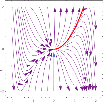
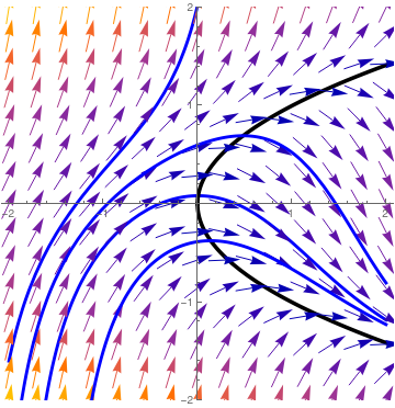
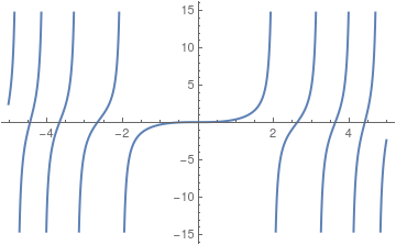
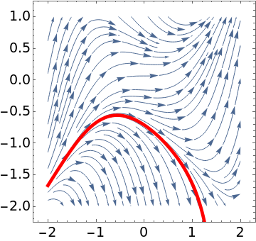
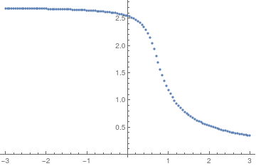
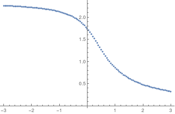
We plot the nullcline (in black) y² = x and phase portrait) for the Riccati equation
\( y' = y^2 - x. \)
The nullcline and phase portrait for the Riccati equation (7.1).
Mathematica code
The Wolfram language has a built-in function, Quiet{ ], which suppresses error messages. In the code below, that function is used to suppress three error messages:
--- NDSolve: At x == 0.5003014382357801' step size is effectively zero
and
--- NDSolve: At x == -1.57885, step size is effectively zero
--- InterpolatingFunction: Input value {-1.99992} lies outside the range
The alert reader is urged to remove the Quiet[ ] wrappers added to the code below to reveal the error messages and research the reason for these warnings. It is possible that these warnings are trivial, just reminders of weakness in numerical vs. analytical methods. But more serious pathological problems may be at the root of these messages. Learning about these can be very illuminating.
Later in this notebook and on the companion webpage, the practice of using or failing to use Quiet[ ] shall be governed by the context and the contribution to clarity either choice may provide.
Since the polynomial Δ = 4x for Eq.(7.1) is of first degree, this Riccati equation has no polynomial solution. However, Euler's substitution y = −u′/u reduces the given Riccati equation to a linear differential equation:
\[
u'' + x\, u = 0 .
\tag{7.2}
\]
Its general solution is expressed through Airy functions (these functions are discussed in APMA0340 course, see section)
\[
u(x) = c_1 \mbox{Ai}\left( (-1)^{1/3} x \right) + c_2 \mbox{Bi}\left( (-1)^{1/3} x \right)
\tag{7.3}
\]
Mathematica is capable to solve the Riccati equation (7.1), but it expresses it through Bessel functions of pure imaginary argument.
DSolve[y'[x] == (y[x])^2 - x, y[x], x]
BesselJ[-(4/3), 2/3 I x^(3/2)] C[1] +
BesselJ[2/3, 2/3 I x^(3/2)] C[
1]))/(2 x (BesselJ[1/3, 2/3 I x^(3/2)] +
BesselJ[-(1/3), 2/3 I x^(3/2)] C[1]))}}
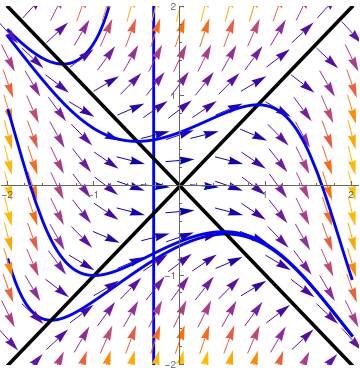
Now we consider another Riccati equation
\[
y' + \left( 2 x^2 -1 \right) y = y^2 + 4x .
\tag{7.4}
\]
Then the polynomial
\[
\Delta = \left( 2 x^2 -1 \right)^2 + 2x - 4\,4x = 4 x^4 - 4 x^2 -12x +1
\]
is of degree 4 (even). So we expect that the Riccati equation (7.4) may have a polynomial solution
\[
y = a\,x^2 + b\,x + c \qquad \Longrightarrow \qquad y' = 2a\,x + b .
\]
Substituting this polynomial into Eq.(7.4), and equating coefficients of like powers, we obtain
the solution y = 2 x² − 1.
Mathematica also knows the solution
However, finding a polynomial solution may become problematic when the function f(x) = −x will be replaced by another polynomial, say f(x) = x².
■
End of Example 7
An equation of the first order and first degree
\[
y' = A(x) + B(x)\, y^2 , \qquad B(x) \ne 0,
\tag{2}
\]
is called the Riccati equation in normal form.
From previous discussion, we know that with appropriate substitution, the coefficient B(x) can always be reduced to 1, which leads to to normal form
\[
y' = A(x) + y^2 .
\tag{3}
\]
Riccati himself was concerned
with solutions to so called specialequation with constant coefficients
where n, 𝑎, and b are real numbers.
The special Riccati equation \eqref{EqRiccati.6} can be linearized by Euler's substitution \( y' = -u' /(au) . \) This yields
\[
\frac{{\text d}^2 u}{{\text d} x^2} + \left( ab \right) x^n u = 0 .
\]
Multiplying both sides of this linear equation by x², we obtain a non-standard Bessel equation that is considered in section of the second course APMA0340:
where \( q= 1+ n/2 , \quad 2q = n+2 = \nu^{-1} , \ \) and Jν(t), Yν(t) are Bessel functions of first and second kind, respectively, ,
while Iν(t), Kν(t) are modified Bessel functions. Note that the general solution depends on the
ratio c₁/c₂ (if c₂ ≠ 0) or c₂/c₁ (if c₁ ≠ 0) of two arbitrary constants c₁ and c₂.
where C₁ and C₂ are arbitrary constants (not both zero).
The solution of the Riccati equation subject to the homogeneous initial condition y(0) = 0 is known from Eq.(8.2):
Now we test how Mathematica handles discontinuities (singular points) while solving the initial value problems numerically. It turns out that NDSolve command provides a very accurate approximation of the critical point:
The initial value problem \( y' = y^2 + x^2 , \quad y(0) =0 \) has two forms of solutions \eqref{EqRiccati.6}
expressed through Bessel functions of the first kind only:
To convince you that this is the same solution presented in another form, we do two things. First, we expand the above solution into Maclarin series and compare it with true expansion. Second, we verify that our function satisfies the given Riccati equation and the initial condition because the solution of such initial value problem is unique.
Theorem 3 (Bernoulli--Liouville). The special Riccati equation
\( y' = a\,y^2 + b\, x^{n} \) can be integrated in closed form via elementary functions if and only if
From Eq.(9), we know that the general solution of the special Riccati equation (7) is expressed through Bessel functions (first and second kind) of index ν = 2/(n + 2). From section of the second course APMA0340, we know that Bessel functions are expressed through elementary functions only when their index is half integer. Solving equation 2/(n + 2) == 1/2 + k, we obtain the required formula.
Solve[1/(n + 2) == k-1/2, n]
{{n -> -((4 (-1 + k))/(-1 + 2 k))}}
▣
In the same volume of Acta Eruditorum containing the famous Riccati's equation, there was published an article by 24-year-old Daniel Bernoulli, in which he wrote that all three members of the Bernoulli family (Nicolas, Johann, and himself) independently had found conditions for the parameter n under which the special Riccati equation \eqref{EqRiccati.6} is integrable in elementary functions:
\[
\frac{n}{2n + 4} \quad \mbox{is an integer}.
\tag{11a}
\]
This formula is actually equivalent to Eq.(11). When k → ∞ in Eq.(11), we obtain the value of n to be −2, for which the special Riccati equation \eqref{EqRiccati.6} is also integrable in elementary functions. In 1841, J. Liouville proved that the special Riccati equation \eqref{EqRiccati.6} is not integrable in elementary functions for any other values of parameter n.
▣
Example 10:
We check the conclusion of Theorem 3 with a series particular cases. In order to simplify our job, we employ Mathematica.
Setting k = 0 in Eq.(11), we get n = −4. Then the special Riccati equation becomes
\[
y' = \frac{{\text d}y}{{\text d}x} = y^2 + \frac{4}{x^4} .
\tag{10.1}
\]
So the general solution of Eq.(10.1) is
\[
y = \frac{\left( x\,c -2 \right) \sin \left( \frac{2}{x} \right) - \left( x + 2c \right) \cos \left( \frac{2}{x} \right)}{x^2 \cos \left( \frac{2}{x} \right) - x^2 c\,\sin \left( \frac{2}{x} \right)} .
\]
mysol[x_, a_, b_, n_] := Module[{k = 1 + n/2, w, y},
w = Sqrt[
x]*(C[1]*BesselJ[1/(2*k), 1/k*Sqrt[a*b]*x^k] +
C[2]*BesselY[1/(2*k), 1/k*Sqrt[a*b]*x^k]);
y = Simplify[-D[w, x]/(a*w)];
y = y /. C[1] -> 1;
y
];
a = 1; b = 1; n = -4;
ode = y'[x] == a*y[x]^2 + b*x^n;
sol = mysol[x, a, b, n]
ode /. y -> Function[{x}, Evaluate[sol]];
sol = mysol[x, 1, 4, -4]
However, if you try to solve
\[
y' = y^2 + \frac{1}{x^2} ,
\]
Mathematica will provide you a complex-valued answer:
\[
y = \frac{{\bf j} \left( - x^{{\bf j}\sqrt{3}} - 3\,c \right) \sqrt{3} + 3\,x^{{\bf j}\sqrt{3}} + 3\,c}{2 \left( {\bf j}\,x^{{\bf j} \sqrt{3}} \sqrt{3} - 3\,c \right) x} ,
\]
where c is an arbitrary constant and j is the unit imaginary vector on the complex plane ℂ so j² = −1. The complex-valued solution is obtained from formula (8) because \( \displaystyle \quad k = - \frac{1}{2} + {\bf j} \,\frac{\sqrt{3}}{2} \quad \) is a solution of quadratic equation k² + k + 1 = 0.
When n = 0, we get a separable equation
\[
y' = y^2 +1 \qquad \Longrightarrow \qquad y = \tan \left( x + c \right) ,
\]
where c is an arbitrary constant.
Now we set k = 2 in Eq.(11), so n = −4/3, and we have
\[
y' = \frac{{\text d}y}{{\text d}x} = y^2 + \frac{1}{x^{4/3}} .
\tag{10.2}
\]
Its solution is
\[
y = x^{-1/3} \,\frac{3\,\sin \left( 3\,x^{1/3} \right) - 3c\,\cos \left( 3\,x^{1/3} \right)}{\left( 3 x^{1/3} + c \right) \cos \left( 3\,x^{1/3} \right) + \left( 3 x^{1/3} c -1 \right) \sin \left( 3\,x^{1/3} \right)} .
\]
If we set k = −1 in Eq.(11), so n = −8/3, and we have
\[
y' = \frac{{\text d}y}{{\text d}x} = y^2 + \frac{1}{x^{8/3}} .
\tag{10.3}
\]
Its solution is
\[
y = x^{-4/3}\,\frac{\left( 3 - x^{2/3} + 3 x^{1/3} c \right) \cos \left( 3\,x^{-1/3} \right) - \left( 3 x^{1/3} -3c + x^{2/3} c \right) \sin \left( 3\,x^{-1/3} \right)}{\left( x^{1/3} -3c \right) \cos \left( 3\,x^{-1/3} \right) + \left( 3 + x^{1/3} c \right) \sin \left( 3\,x^{-1/3} \right)} .
\]
A similar situation is observed when one of the coefficients (𝑎 or b or both in Eq.(7)) is negative. For instance, the special Riccati equation
\[
y' = \frac{{\text d}y}{{\text d}x} = y^2 - \frac{1}{x^{8/3}} .
\tag{10.6}
\]
has the general solution
\[
y = x^{-4/3}\, \frac{\left( 3 x^{1/3} c + 3{\bf j} + x^{2/3} {\bf j} \right) \cosh \left( 3 x^{-1/3} \right) - \left( 3\,{\bf j} x^{1/3} + \left( 3 + x^{2/3} \right) c \right) \sinh \left( 3 x^{-1/3} \right) }{\left( 3\,{\bf j} + x^{1/3} \right) \sinh \left( 3 x^{-1/3} \right) - \left( 3\,c + {\bf j}\,x^{1/3} \right) \cosh \left( 3 x^{-1/3} \right) } ,
\]
where j is the unit imaginary vector on the complex plane ℂ so j² = −1.
Because the calculus of variations and optimal control theory serve as the main source for obtaining and interpreting the differential (matrix) Riccati equation, our first example must be devoted to this topic.
Classical calculus of variations originated in 1696 when the famous troublemaker and genius Johann Bernoulli (1667--1748) posed a mathematical challenge. It is known as the brachistochrone problem that asks what shape a curve should be between two points at different elevations so that a frictionless object sliding down it under gravity would reach the lower point in the shortest possible time. Although the brachistochrone problem is discussed in detain in section from the fourth part of this tutorial, it surves as an motivation to the calculus of variation.
A very clever contribution to the Wolfram Demonstration Project entitled "The Great Brachistochrone Race" may be found at this link. The code that follows is a slightly modified version that produced the graphic you see next which shows that the shortest time to traverse between two points is not a straight line when gravity is involved.
Before we formulate optimization problems, it is convenient to introduce the following well-known notation: ℭm([t₀, t₁], ℝn) for the vector space of all continuous vector-valued functions having m first continuous derivatives (in our case, m = 2), so when f : [t₀, t₁] → ℝn is a smooth function, we abbreviate it as f ∈ ℭm (for simplicity). However, for optimization problems, we use its subset ℳ ⊂ ℭm of functions satisfying fixed boundary conditions
\[
f \left( t_0 \right) = \mathbf{a} , \qquad f \left( t_1 \right) = \mathbf{b} ,
\]
where a and b are two given points in ℝn. With this assumption, ℳ is not a vector space.
We also use notation ℭm0 the vector space of all m times differentiable functions that vanish at endpoints: f(t₀) = f(t₁) = 0.
In general, an optimization problem consists of maximizing or minimizing an integral expression known as an action functional
where L ∈ ℭ²([t₀, t₁], ℝn, ℝn) is twice continuously differentiable function. Although three variable (t, x, v) in L are independent, these variables are coupled together because they are evaluated at the same time in the action functional. In mechanics, L is referred to as the Lagrangian (L = K − Π, the difference of the kinetic energy and potential energy). When row vector x is given in generalized coordinates as a contravariant vector in ℝn, x(t) = [q¹, q², … , qn], the action functional is written as
We say that a weak minimum is attained for a curve x✶(·) ∈ ℳ if there exists δ > 0 such that for any x(·) ∈ ℳ ⊂ ℭ¹([t₀, t₁]) with ∥x✶(·) − x(·)∥ < δ, x(t₀) = a and x(t₁) = b, the inequality J(x(·)) ≥ J(x✶(·)) holds.
A function x✶(·) ∈ ℳ is a global minimizer if J(x✶) ≤ J(x) for all x ∈ ℳ. If ≤ is replaced by <, it is called a strict minimizer.
Let f : Ω → ℝ be a smooth function (having at least three first derivatives), where Ω ⊆ ℝn. For given two (contrarian) vectors x = [x¹, x², … , xn] and η = [η¹, η², … , ηn], Taylor's multivariable theorem implies, for ε near zero,
As usual, we denot partial derivatives with subscripys:
\( \displaystyle \quad \partial_i f = f_{x^i} = \frac{\partial f}{\partial x^i} \quad\mbox{and} \quad \partial_{i,j}f = f_{x^i x^j} = \frac{\partial^2 f}{\partial x^i x^j} . \quad \) Since the Hessian is a symmetric matrix, it does not matter how you evaluate the inner product (either multiply the Hessian matrix from left or from right before evaluating the inner product).
If x✶ is a critical point of f, then ∇f(x✶) = 0 and we have
In particular, if x✶ is a local minimum, then the inner product ⟨η∣H∣η⟩ > 0 for η ≠ 0.
(in this case, we say that matrix H is positive definite). In two-dimensional case this condition is equivalent to
where ε is a small parameter and η = [η¹, η², … , ηn] ∈ ℭ20([t₀, t₁], ℝn) is a test function vanishing at end points, η(t₀) = η(t₁) = 0. For velocities we have the corresponding relation
We then back to a calculus problem, where x✶ ∈ ℳ is a local minimizer of J(·) if and only if 0 is
a local minimum of ϕ(·) because J(x✶) = ϕ(0). Note that the theorem on differentiability of an integral with respect to a parameter and the the assumption L ∈ ℭ2 imply that the function ϕ(ε) is twice differentiable in ε. Expanding ϕ(·) into truncated Taylor's series, we obtain
is its second order variation. The action J is extremal if δJ = 0 for any deformation η ∈ ℭ20([t₀, t₁], ℝn) that keeps endpoints fixed to zero.
So the optimality condition of an extreme curve x✶ of J(x) is characterized as δJ = 0. In order to extract conditions on the Lagrangian L(t, x, v) that guarantee extremal x✶ of the action, we need the following lemma that was proved by the German physiologist Emil Heinrich du Bois-Reymond (1818--1896) in 1879.
Lemma 2 (du Bois-Reymond):
Let \( \displaystyle \quad a(t), \ b(t), b'(t) \in ℭ([t_0 , t_1 ], \mathbb{R}^n ) , \quad \) and let the condition
\[
\int_{t_0}^{t_1} \left[ a(t)\,h(t) + b(t)\, \dot{h} (t) \right] {\text d}t = 0
\]
hold for any test function h ∈ ℭ10([t₀, t₁], ℝn). Then the function b(t) satisfy the equation
\[
\frac{\text d}{{\text d}t}\, b(t) = a(t) .
\]
Let A(t) denote any an arbitrary primitive of the function 𝑎(t), i.e., \( \displaystyle \quad A(t) = \int_{t_0}^t a( \tau )\,{\text d}\tau + K, \quad \) for some constant K. Integrating the first summand by parts and taking into account property of h to vanish at end points, we obtain
\[
\int_{t_0}^{t_1} \left[ -A(t) + b(t) \right] \dot{h}(t)\,{\text d}t = 0
\tag{E.1}
\]
(for any choice of constant K). We now choose h(t) such that
\[
h(t) = \int_{t_0}^t \left[ -A(\tau ) + b(\tau ) \right] {\text d}\tau .
\]
Then h(t₀) = 0 and condition h(t₁) = 0 is ensured by the choice of constant K. Substituting h(t) into Eq.(E.1), we get
\[
\int_{t_0}^{t_1} \left[ -A(t) + b(t) \right]^2 {\text d} t = 0.
\]
Hence, A(t) = b(t).
Changing the order of integration and differentiation with respect to parameter ε, we find
where H10([t₀, t₁], ℝn) is the closer of ℭ10([t₀, t₁], ℝn), which can be converted into the Sobolev space.
Since coordinates q¹, q², … , qn and their derivatives are independent, we apply the du Bois-Reymond lemma to each component to obtain a system of differential equations
This system of equations is referred to as the Euler equations or Euler--Lagrange equations. Solutions of the system of n ordinary differential equations of the second order \eqref{EqRiccati.14} must belong to the set ℳ ⊂ ℭ2; therefore, solution curves should have fixed endpoints.
When the lagrangian is independent of t,
which is called autonomous, we have the conservation of Hamiltonian
\[
H \left( \mathbf{x} , \dot{\mathbf{x}} \right) = \sum_{i=1}^n L_{\dot{q}^i}\,\dot{q}^i - L \left( \mathbf{x} , \dot{\mathbf{x}} \right) ,
\]
which is an integral of the Euler equations \eqref{EqRiccati.14}.
Example 12:
In Cartesian coordinates, we set the initial point to be the origin and choose the vertical direction to ne downward. Let y = y(x) be the equation of the brachistochrone curve. By the energy conservation law, the speed of the bosy at the point (x, y(x)) is the same as in the free-fall motion from the height y(x), i.e., \( \displaystyle \quad v = \sqrt{2g\,y(x)} . \quad \) Therefore, integrating along the curve y = y(x), we obtain the time of motion
\[
\int \frac{{\text d}s}{v} = \int_0^x \frac{\sqrt{1 + \left( \dot{y} (x) \right)^2}}{\sqrt{2g\,y(x)}} \,{\text d} x .
\]
Hence, the problem is to choose a function y = y(x) such that the conditions y(0) = 0 and y(x₀) = y₀ are satisfied and functional above has the minimum value.
The corresponding acting functional is
\[
J\left( y(\cdot ) \right) = \int_{0}^{b} \frac{\sqrt{1 + \dot{y}^2}}{\sqrt{y}}\, {\text d} t ,
\tag{12.1}
\]
where \( \displaystyle \quad \dot{y} = {\text d}y/{\text d}t \quad \) is the derivative of function y, which is considered as twice continuously differentiable function, abbreviated as L ∈ ℭ²([0, b] × ℝ¹ × ℝ¹). Also, it is assumed that function y = y(x) in Eq.(12.1) has fixed endpoints:
\[
y \left( 0 \right) = 0 , \qquad y \left( \ell \right) = b .
\]
Then
\[
L_y = -\frac{\sqrt{1 + \dot{y}^2}}{2\sqrt{y^3}} , \qquad L_{\dot{y}} = \frac{\dot{y}}{\sqrt{1 + \dot{y}^2}\, \sqrt{y}} .
\]
With this in hands, we evaluate the derivative
\[
\frac{\text d}{{\text d}x}\, L_{\dot{y}} = \frac{\ddot{y}}{\sqrt{\left( 1 + \dot{y}^2 \right)^3}\,\sqrt{y}} - \frac{\dot{y}^2}{1 \sqrt{1 + \dot{y}^2}\,\sqrt{y^3}} .
\]
Hence, the Euler equation becomes
\[
- \frac{\ddot{y}}{\sqrt{\left( 1 + \dot{y}^2 \right)^3}\,\sqrt{y}} + \frac{\dot{y}^2}{1 \sqrt{1 + \dot{y}^2}\,\sqrt{y^3}} - \frac{\sqrt{1 + \dot{y}^2}}{2\sqrt{y^3}} = 0
\]
or
\[
2y\,\ddot{y} + \dot{y}^2 + 1 = 0
\]
Since this equation does not contain the independent variable, we make substitution
\[
\dot{y} = p(x) , \qquad \ddot{y} = p\.\frac{{\text d}p}{{\text d}y} .
\]
This yields
\[
2yp\,\frac{{\text d}p}{{\text d}y} + p^2 + 1 = 0 \qquad \Longrightarrow \qquad \frac{2p}{p^2 + 1}\,{\text d}p = - \frac{{\text d}y}{y} .
\]
Integrating both sides, we obtain
\[
\ln \left( 1 + p^2 \right) = \ln \frac{C}{|y|} \qquad \Longrightarrow \qquad p = \pm \sqrt{\frac{C}{y} -1} .
\]
Choosing the plus sign in the latter, we get
\[
\frac{{\text d}y}{\sqrt{C/|y| -1}} = {\text d}x .
\]
Replacing y with Csin²t, we obtain
\[
x = \int \frac{2C\,\sin t\,\cos t\,{\text d}t}{\sqrt{1/\sin^2 t -1}} = C\,\int 2\,\sin^2 t\,{\text d}t .
\]
Therefore,
\[
\begin{cases}
x &= D + C\,t - C\,\frac{\sin 2t}{2} = \frac{C \left( 2t - \sin 2t \right)}{2} +D , \\
y &= C\,\sin^2 t = \frac{C \left( 1 - \cos 2t \right)}{2} ,
\end{cases}
\]
which is a parametric equation of cycloid.
Stricktly speaking, our derivation of extremal curve for the brachistochrone problem is not accurate because of existence of a singular point y = 0. For its proof, see
Young, L., Lectures on the Calculus of Variations and Optimal Theory, Philadelphia, W.B. Saunders Co. 1969.
𝑎
■
End of Example 12
The sign of the second variation δ²J is related to the stability of solutions of the Euler--Lagrange equations \eqref{EqRiccati.14}. If δ²J > 0 for all deformations, then the second deviation is called positive definite. In this case, we have a minimum; if δ²J < 0, we have a maximum; if δ²J = 0 for some deformations, we have a degenerate extremum. However, to ensure positivity of the second variation, we restrict ourselves to deformations in which first derivatives are also kept fixed to zero. Then
Taking n = 1 will substantially simplify exposition without loosing any key idea of observation---matrix Riccati equation is a topic of the second course, APMA0340. In the case of a scalar-valued function, the second deviation can be written as
because the strong Legendre condition p(t) > 0 is assumed to be held. The second variation δ²J is called positive definite if δ²J(y, η) > 0 for η ≠ 0 and η ∈ H10.
Unfortunately, the Riccati equation \eqref{EqRiccati.16} may have no solution that is continuous on the whole interval [t₀, t₁]
Example 13:
Let the acting functional be
\[
J = \int_0^{\ell} \left[ \dot{y}^2 - y^2 (t) \right] {\text d} t , \qquad y(0) = y(\ell ) = 0 ,
\]
for some fixed positive ℓ. Expanding the scalar function
\[
\phi (\varepsilon ) = \int_0^{\ell} \left[ \left( \dot{x}^{\ast} + \varepsilon\,\dot{\eta} \right)^2 - \left( x^{\ast} (t) + \varepsilon\,\eta \right)^2 \right] {\text d} t ,
\]
where x✶ is the minimizer (unknwn yet) of teh functional J, we obtain
It turns out, with η(0) = η(ℓ) = 0, one always has the Poincaré inequality
\[
\int_0^{\ell} \eta^2 {\text d}t \leqslant \frac{\ell^2}{\pi^2} \int_0^{\ell} \dot{\eta}^2 {\text d}t .
\]
Hence, the second deviation can be estimated from below
\[
\delta^2 J = 4 \int_{0}^{\ell} \left( \dot{\eta}^2 - \eta^2 \right) {\text d} t \ge 4 \left( 1 - \frac{\ell^2}{\pi^2} \right) \int_0^{\ell} \dot{\eta}^2 {\text d} t .
\]
If ℓ ≤ π, the second deviation δ²J ≥ 0 for any test function η. Therefore, the
necessary condition for a minimum is met for any extremal x✶, and J cannot
have a local maximum.
If ℓ ≥ π, we can choose a sequence of test functions
\( \displaystyle \quad \eta_n (t) = \sin\frac{n\pi t}{\ell} , \quad n = 1, 2, \ldots . \quad \) Then every member of this sequence satisfies the homogeneous boundary conditions. Using double angle formula, we get
\[
\delta^2 J \left( \eta_n \right) / 4 = \int_0^{\ell} \left( \frac{n^2 \pi^2}{\ell^2}\,\cos^2 \frac{n\pi t}{\ell} - \sin^2 \frac{n\pi t}{\ell} \right) {\text d} t = \frac{n^2 \pi^2 - \ell^2}{2\,\ell^2} .
\]
Thus, for n = 1, the second deviation is less than zero, but for any n with n²ℓ² > ℓ², the second deviation is positive. Therefore, any extremal of J cannot be a local
minimum or local maximum.
The corresponding Riccati equation becomes \( \displaystyle \quad \dot{w} = 1 + w^2 . \quad \) Separation of variables yields w = tan(t + C). If the length of the closed interval [t₀, t₁] is greater than π, then w(t) has a point of discontinuity on this interval.
𝑎
■
End of Example 13
Now we turn to another applications of Riccati's equations in Mathematical finance. In particular, we consider the famous Cox--Ingersoll--Ross (CIR) model, which provides one of the best known models of stochastic interest rates.
Example 14:
We first introduce a particular class of stochastic interest-rate models known as affine term structure models. Affine models have certain attractive properties in terms of their tractability. We need a couple of concepts from finance to proceed. The first concept is that of a zero-coupon bond. A zero-coupon bond is a contract which will pay one unit, with certainty, at a prespecified future date. If the current time is t and the future payment will occur at time T > t, then we denote the current price of the zero-coupon
bond by P(t, T). The market prices for these bonds can be obtained from traded market instruments. The short rate of interest can be defined in terms of zero-coupon bond prices. Let us first define the function f(t, T) by
\[
f(t, T) = - \frac{\partial \log\,P(t, T)}{\partial T} .
\]
This function f(t, T) is known as the forward rate. The short rate r(t) is defined as the
limiting value of f(t, T) as T tends to t:
\[
r(t) = \lim_{T\to t} f(t, T) .
\]
The short rate can be thought of as the limiting interest rate on a bond where we let the time to maturity tend to zero (for detail, see Duffie).
The starting point for several popular stochastic interest-rate models is to assume that the short rate dynamics are governed by a stochastic differential equation involving one or more state variables and a number of structural
parameters. However, we assume that there is only one such state variable. Such models are known as one factor models. Under a special class of such models, known as the one factor affine class, the resulting model prices for the zero-coupon bonds are exponential-linear functions of the short rate of interest.
Assume the short-term interest rate is described by the following
stochastic differential equation
\[
{\text d}r = \mu (t, r)\,{\text d}t + \sigma (t, r)\,{\text d}W_t ,
\]
where Wt is a standard Brownian motion under the risk-neutral equivalent measure (for detail, see Duffie 1996).
The definition of an affine term structure model is that P(t, T) has the exponential form
\[
P(t, T) = \exp \left\{ A(t, T) - B(t, T)\,r(t) \right\}
\]
and thus the yield \( \displaystyle \quad y(t, T) = - \frac{\log P(t, T)}{T-t} \quad \) is a linear function of r(t). Duffie–Kan’s result is that P(t, T) is exponential-affine if and only if the diffusion µ and the volatility σ have
the form
\[
\mu (t, r) = \alpha (t)\,r + \beta (t) , \qquad \sigma (t, r) = +\sqrt{\gamma (t)\, r + \delta (t)} .
\]
Moreover, the coefficients A(t, T), B(t, T) are determined by the following ordinary differential equations
\[
\dot{B} (t, T) = \frac{\gamma (t)}{2}\, B(t, T)^2 - \alpha (t)\,B(t, T) - 1,
\tag{14.1}
\]
and
\[
\dot{A} (t, T) = \beta (t)\,B(t, T) - \frac{\gamma (t)}{2}\, B(t, T)^2 .
\tag{14.2}
\]
The first equation (14.1) for B(t, T) is the Riccati equation and the second one is a problem from calculus when derivative is given. So function A(t, T) is obtained by integration
because its right-hand side in known from the first equation (14.1) subject that this Riccati equation has been solved.
A note on theory vs. practice
While the equations in Example 14 are elegant and accurate, they also represent a limitation inherent in modeling reality with mathematics. The use of the Riccati equation for modeling interest rates is, at best, naive. Interest rates contain nearly universal information about the financial world, resembling therein a kind of chaos. As such it is too much to require any single equation to produce useful predictions. Below is a fixed version of an animation you may obtain at the Wolfram repository for this material or at the link in the references. You can move the slider to reveal more than 70 years of monthly term structure plots. The shapes vary considerably and at times dramatically. Entire societies rise and fall with the change in the shape of these plots. Issuance of some maturities changes over time. Some shapes have unique names as the drop down menu illustrates. Politics play a role. The plot is red during Republican administrations; blue for Democrat.
Roll, Richard, The Behavior of Interest Rates, The Application of the Efficient Market Model to U.S. Treasury Bills, Basic Books, Inc., New York, New York (1970).
Rosenlicht, M. (1973). An analogue of l’Hospitals rule. Proc. AMS, 37, 369–373.
■
End of Example 14
Show that if two solutions y₁(x) and y₂(x) of the Riccati equation (1) are known, the general solution is
\[
\frac{y - y_1}{y - y_2} = c\,\exp \left\{ \int g(x) \left( y_1 - y_2 \right) {\text d} x \right\} ,
\]
Show that if three solutions of the Riccati equation are known, say y₁(x), y₂(x), and y₃(x), then the general solution is
\[
\frac{\left( y - y_1 \right) \left( y_2 - y_3 \right)}{\left( y - y_2 \right) \left( y_1 - y_3 \right)} = c .
\]
Show that if y₁(x), y₂(x), y₃(x), and y₄(x) are any four different solutions of the Riccati equation (1), then
\[
\frac{y_1 = y_3}{y_1 - y_2} \cdot \frac{y_4 - y_2}{y_4 - y_3} = \mbox{constant} .
\]
Hint: First show that u = (y₁ − y₂)−1 is a solution of the linear differential equation u′ - (p − 2gy₁)u + g = 0. Similarly, u₁ = (y₃ − y₂)−1 and u₃ = (y₄ − y₂)−1 are solutions of this differential equation.
Solve the Riccati equation y′ + y² = 1 + x².
Find all solutions of the Riccati equation y′ − y = 2 − y².
Solve the Riccati equation y′ + 2y = xy² + 4(1 − x). Hint: Function y = 2 is a particular solution.
Find all solutions of the Riccati equation y′ − 2y + y² + 2 = 0.
Solve the Riccati equation \( \displaystyle \quad \frac{{\text d}y}{{\text d}x} = \frac{y^2}{x-1} - \frac{x\,y}{x-1} +1 \quad \) by noting that y = 1 and y = x are its solutions.
Solve the Riccati equation x²y′ − 2x y + x²y² + 2 = 0.
Solve the Riccati equation x²y′ − 3x y + y² + 2x² = 0.
Solve the Riccati equation y′ + y² + b/x² = 0 with a constant b.
Solve the Riccati equation xy′ − y + xy² + x³ = 0.
Akinyemi, L., Erebholo, F., Palamara, V., Oluwasegun, K., A Study of Nonlinear Riccati Equation and Its Applications to Multi-dimensional Nonlinear Evolution Equations, Qualitative Theory of Dynamical Systems, 2024, № S1; https://doi.org/10.1007/s12346-024-01137-2
Bolza, O, Vorlesungen uber Variationsrechnung, Teubner, Leipzig and Berlin, 1909.
Haaheim, D.R. and Stein, F.M.,
Methods of Solution of the Riccati Differential Equation,
Mathematics Magazine, 1969,
Vol. 42, No. 5, pp. 233--240; https://doi.org/10.1080/0025570X.1969.11975969
Kamke, E., Differentialgleichungen: Losungsmethoden und Losungen, I, Gewohnliche Differentialgleichungen, B. G. Teubner,
Leipzig, 1977.
Liouville, J., Remarke nouvelles sur l'équation de Riccati, Journal de Mathématiques Pures et Appliquées, 1841, vol. 6, p. 1--13.
Murphy, G.M., Ordinary Differential Equations and their Solutions, Van Nostrand, Princeton, 1960.
Polyanin, A. and Zaitsev, V.F., Handbook of exact solutions for ordinary differential equations, Second edition,
Chapman and Hall/CRC, 2003.
Riccati, Count J. F., Animadversationes in aequationes differentiales secundi gradus, Actorum Eruditorum quae Lipsiue publicantur. Supplementa, 8 (1724), 66-73.
Translation of the original Latin into English by Ian Bruce.
Robin, W., A new Riccati equation arising in the theory of classical orthogonal polynomials, International Journal of Mathematical Education in Science and Technology, 2003,
Volume 34, 2003 - Issue 1, pp. 31--42. https://doi.org/10.1080/0020739021000018746
Sugai, I., Riccati’s nonlinear differential equation, The American Mathematical Monthly, 69 (1960) 134-139.
Watson, G.N., A Treatise on the Theory of Bessel Functions, Cambridge University Press; 2nd edition, 1995.
Zelikin, M.I., Control Theory and Optimization I: Homogeneous Spaces and the Riccati Equation in the Calculus of Variations (Encyclopaedia of Mathematical Sciences, volume 86), Springer, 2010.
Return to computing page for the first course APMA0330
Return to computing page for the second course APMA0340
Return to Mathematica tutorial for the first course APMA0330
Return to Mathematica tutorial for the second course APMA0340
Return to the main page for the course APMA0330
Return to the main page for the course APMA0340
Return to Part II of the course APMA0330