Preface
This section discusses a simplified version of the Adomian decomposition method first concept of which was proposed by Randolf Rach in 1989 that was crystallized later in a paper published with his colleagues G. Adomian and R.E. Meyers. That is way this technique is frequently referred to as the Rach--Adomian--Meyers modified decomposition method (MDM for short). Initially, this method was applied to power series expansions, which was based on the nonlinear transformation of series by the Adomian--Rach Theorem. Similar to the Runge--Kutta methods, the MDM can be implemented in numerical integration of differential equations by one-step methods. In case of polynomials or power series, it shows the advantage in speed and accuracy of calculations when at each step the Adomian decomposition method allows one to perform explicit evaluations.
Return to computing page for the second course APMA0340
Return to Mathematica tutorial for the second course APMA0340
Return to the main page for the course APMA0330
Return to the main page for the course APMA0340
Return to Part IV of the course APMA0330
Glossary
Forced Vibrations
See http://www.sharetechnote.com/html/DE_Modeling_Example_SpringMass.html#SingleSpring_SimpleHarmonic_Vert_Damp_Force http://www.sharetechnote.com/html/DE_Modeling_Example_SpringMass.html#Single_Spring_with_ExternalForce
This section presents the situation in which a periodic external force is applied to a spring-mass system.
Example: Suppose that the motion of a certain spring-mass system satisfies the differential equation
Since our solution required many steps, we show akternative way to find the solution using the Laplace transform. Upon application of the Laplace transformation to the given inital value problem, we reduce it to an algebraic problem:
FullSimplify[ComplexExpand[%]]
FullSimplify[ComplexExpand[%]]
FullSimplify[%]
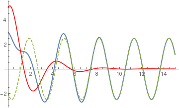
It is important to note that the solution consists of two distinct parts. the terms containing the exponential factor \( e^{-t/2} \) rapidly approach zero. It is customary to call these terms transient. the remaining terms involve only sines and cosines, so they represent an oscillation that last indefinitly. We refer to them as a steady state. The transient part comes from the solution of the corresponding homogeneous equation \( 4\,\ddot{y} +4\,\dot{y} + 10\,y(t) = 0 \) subject to the given inital conditions. It is presented on the graph by red curve. The steady state is the particular solution of the driven equation \( 4\,\ddot{y} +4\,\dot{y} + 10\,y(t) = 25\,\sin \left( 2\,t \right) . \) Shortly, the transient solution vanishes and the full solution is essentially indistinguishable from the steady state.
yp[t_] = E^(-t/2) (5 Cos[(3 t)/2] + 3 Sin[(3 t)/2])
yh[t_] = -2 Cos[2 t] - 3 Cos[t] Sin[t]
Plot[{y[t], yp[t], yh[t]}, {t, 0, 15}, PlotStyle -> {Thick, Red, Dashed}]
- Cveticanin, L.,Strongly Nonlinear Oscillators–Analytical Solutions, Undergraduate Lecture Notes in Physics, Springer, 2014.
- Cveticanin, L., Luburic, U.K., Mester, G., Periodic Motion in an Excited and Damped Cubic Nonlinear Oscillator, Mathematical Problems in Engineering, 2018, Volume 2018, Article ID 3841926, 6 pages; https://doi.org/10.1155/2018/3841926
- Cveticanin, L., Mester, G., Biro, I., Parameter influence on the harmonically excited Duffing oscillator, Acta Polytechnica Hungarica, vol. 11, no. 5, pp. 145–160, 2014.
- Holmes, P., A nonlinear oscillator with a strange attractor, Philosophical Transactions of the Royal Society A: mathematical, Physical, and Engineering Sciences, 1997, Volume 292, Issue 1394, pp. https://doi.org/10.1098/rsta.1979.0068
- Hsu, C.S., On the application of elliptic functions in non-linear forced oscillations, Quarterly of Applied Mathematics, vol. 17, pp. 393–407, 1959/1960.
Return to Mathematica page
Return to the main page (APMA0330)
Return to the Part 1 (Plotting)
Return to the Part 2 (First Order ODEs)
Return to the Part 3 (Numerical Methods)
Return to the Part 4 (Second and Higher Order ODEs)
Return to the Part 5 (Series and Recurrences)
Return to the Part 6 (Laplace Transform)
Return to the Part 7 (Boundary Value Problems)