Return to computing page for the first course APMA0330
Return to computing page for the second course APMA0340
Return to computing page for the fourth course APMA0360
Return to Mathematica tutorial for the first course APMA0330
Return to Mathematica tutorial for the second course APMA0340
Return to Mathematica tutorial for the fourth course APMA0360
Return to the main page for the course APMA0330
Return to the main page for the course APMA0340
Return to the main page for the course APMA0360
The fundamental importance of existence theorems for initial value problems (IVPs for short) hardly needs justification. Historically, proofs of these theorems were divided into two categories. The first one employed Cauchy--Lipschitz method and it is based on constructing Euler's polygon approximations (Tonelli sequences). This approach guarantees only existence of solutions, but not its uniqueness. The Euler--Cauchy--Lipschitz method is hard to call constructive and it gives mostly theoretical justification.
Another kind of proofs are based on transferring the given initial value problem (with unbounded differential operator) into an equivalent integral equation that allows one to reformulate the IVP in terms of bounded operator (integral one). Then such integral equation is solved by successive approximations, credited to E. Picard. It is proved that such successive approximations converge to a true solution and its solution is unique. Although practical application of Picard's iteration scheme is limited, it provides a constructive proof of required solution to the IVP. This is the main reason why iteration method is so popular.
Now there are known many generalizations of these two approaches (identified with names Peano and Picard, respectively). However, they involve more sophisticated results, namely fixed point theorems in infinite dimensional function spaces; so we do not pursue this direction.
An ordinary differential equation may have no solution, unique solution or infinitely many solutions. For instance, \( y'^2 + y^2 + 4 =0,
\quad y(0) =3 \) has no solution. The ODE \( y' =
x^2 +y, \quad y(0) =-2 \) has the unique solution
\( y = -2-2x-x^2 , \) whereas the ODE
\(x\,y' = y-2 , \quad y(0) =2 \) has infinitely many solutions y = 2 + αx, where α is any real number.
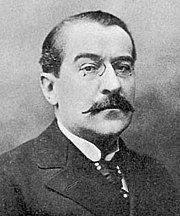
Giuseppe Peano.
Theorem (Peano, 1886)
Let Ω be an open subset of ℝ × ℝ with f : Ω → ℝ to be a continuous bounded function. Then an initial value problem
with (x0, y0) ∈ Ω has a local solution y : Ω → (𝑎, b), whee (𝑎, b) is a neighbourhood of (x0, y0).
This theorem was proved in 1886 by the Italian mathematician Giuseppe Peano (1858--1932).
He employed the Euler--Cauchy--Lipschitz polygon method. The idea of this method consists in considering a suitably chosen Euler polygon as an approximate solution of IVP \eqref{EqExist.1} and in obtaining the solution of IVP \eqref{EqExist.1} as limit of sequences of such approximations. The contemporal proof is presented in the Coddington and Levinson book and it is based on reduction to the integral equation that is later solved by implementing an elegant method due to Tonelli. Peano's theorem does not ensure uniquely determined solution by their initial values.
Giuseppe Peano was a founder of symbolic logic whose interests centered on the foundations of mathematics and on the development of a formal logical language. In 1890, Peano founded the journal Rivista di Matematica, which published its first issue in January 1891. In 1891, Peano started the Formulario Project. It was to be an "Encyclopedia of Mathematics", containing all known formulae and theorems of mathematical science using a standard notation invented by Peano. In 1888, Peano published the book Geometrical Calculus that begins with a chapter on mathematical logic.
In addition to his teaching at the University of Turin, Peano lectured at the Military Academy in Turin in 1886. The following year he discovered and published a method for solving systems of linear differential equations using successive approximations.
Although Émile Picard had independently developed this method, he credited the German mathematician Hermann Schwarz (1843--1921) with its discovery.
It turns out that for existence and uniqueness of solutions to ODEs continuity of the slope function is not sufficient. We need more stronger condition.
A function f from S ⊂ ℝm into ℝn is Lipschitz continuous (also locally Lipschitz continuous) at x ∈ S if there exists a positive constant C such that
for all y ∈ S sufficiently near x from some its neighborhood.
A function f from S ⊂ ℝm into ℝn is called a Lipschitz function if there exists a positive constant C such that the inequality \eqref{EqExis.2} holds for all x, y ∈ S. The smallest constant is sometimes called the (best) Lipschitz constant or the dilation or dilatation.
The following nesting hold:
\[
\mbox{differentiable at $x$} \quad \Longrightarrow \quad \mbox{Lipschitz continuous at $x$} \quad \Longrightarrow \quad \mbox{absolutely continuous} \quad \Longrightarrow \quad \mbox{continuous at $x$}.
\]
In one dimensional case, the geometric intuition tells us if inequality
\( |f(y) - f(x)| \leqslant C\,|y-x| \) holds for x, y ∈ [𝑎, b], then graph of f lies wedged between the line of slope C going through f(𝑎) at 𝑎 and the line of slope −C going through f(𝑎) at 𝑎. This essentially means that the function can't grow too quickly, or wedged too much.
Lemma 1::
Suppose that
f(x) is a real-valued function defines on an interval
[𝑎, b] ⊂ ℝ of not zero length. If its derivative f' = df/dx is bounded on closed interval
[𝑎, b], then f is a Lipschitz function on this interval.
Suppose that M is such that \( | f' (x) | \leqslant M \) for all x ∈ [𝑎, b]. Then for x and y in [𝑎, b], we get from the Mean Value Theorem that
\[
f(y) - f(x) = f' (\xi ) \left( y-x \right)
\]
for some ξ between x and y. Let \( M = \max_{\xi} |f' (\xi )| , \) then
\[
| f(y) - f(x) | \leqslant M \,|y-x| .
\]
Thus, Eq.(1) holds with C = M.
Example 1:
We start with a familiar function: f(x) = |x|. This function is no differentiable in any interval containing the origin. However, f(x) is a Lipschitz function on any finite interval with the Lipschitz constant equal to 1.
The function f = tanx is differentiable at each point from the open interval (−π/2, π/2) and, therefore, Lipschitz continuous at each x ∈ (−π/2, π/2). However, its derivative is unbounded on the open interval, so there is no constant C for inequality (1) to hold. Hence tan(x) is not Lipschitz function on (−π/2, π/2), but it is Lipschitz function on any closed interval [𝑎, b] ⊂ (−π/2, π/2).
is continuous, but its derivative has an essential singularity at the origin, so it is not Lipschitz continuous. This function becomes infinitely steep as x approaches 0 since its derivative becomes infinite. However, it is uniformly continuous.
The main reason of this transformation is to reduce an initial value problem with unbounded derivative operator into a problem with bounded operator such as integration. However, the domain of the Volterra integral operator in right-hand side of Eq.\eqref{EqExis.3} is not defined for all y, so the domain of the operator U has to be determined with care.
Lemma 2::
Let f(x, y) be a real-valued continuous function of the variables x and y. Then any solution of the initial value problem (1) is a solution of the integral equation \eqref{EqExis.3}, and
conversely.
If y(x) satisfies the integral equation \eqref{EqExis.3}, then this function satisfies the initial condition y(x0) = y0. Differentiating both sides of the integral equation and using the fundamental theorem of calculus, we conclude that y(x) is a solution of the given initial value problem (1).
Conversely, the Fundamental Theorem of
the Calculus shows that \( \displaystyle y(x) = y(x_0 ) + \int_{x_0}^x f(y(s),s)\,{\text d}x \) for all continuously differentiable functions y(x). If y(x) satisfies the differential equation \eqref{EqExis.1}, then \( \displaystyle y(x) = y(x_0 ) + \int_{x_0}^x f(y(s),s)\,{\text d}x \) ; if in addition, y(x0) = y0, the integral equation \eqref{EqExis.3} is obtained.
Corollary 1::
The initial value problem (1) has a solution if and only if the inegral equation \eqref{EqExis.3} has a fixed point n class of continuous functions ℭ[x0, h] for some h > x0.
Theorem 2:: Let
f(x,y) be continuous for all (x,y) in open rectangle
\( R= \left\{ (x,y)\,:\, |x-x_0 | < a, \quad |y- y_0 | < b \,\right\} \) and Lipschitz continuous in y, with
constant L independent of x.
Then there exists a unique solution to the initial value problem
\[
y' = f(x,y) , \qquad y(x_0 ) = y_0
\]
on the interval. Moreover, if z(x) is the solution to the same problem with the initial condition \( z(x_0 ) = z_0 , \) then
Theorem (Picard--Lindelöf):
Suppose that a slope function f(x,y) is defined and continuous within an rectangular domain
\[
R = \left\{ (x,y)\,:\, \left\vert x- x_0 \right\vert \le a, \quad
\left\vert y- y_0 \right\vert \le b\right\} , \qquad\mbox{for some positive
constants }a, b.
\]
We also assume that f(x,y) satisfies the following conditions.
The slope function is bounded: \( M = \max_{(x,y) \in R} \, |f(x,y)| . \)
The slope function is Lipschitzcontinuous:
\( |f(x,y) - f(x,z) | \le L\,|y-z| . \) for all
(x,y) from R.
Then for
\[
h = \min \left\{ a, \ \frac{b}{M}, \ \frac{1}{2L} \right\}
\]
the initial value problem
\[
y' = f(x,y), \qquad y(x_0 ) = y_0
\]
has a unique solution y = φ(x) for
\( |x-x_0 | < h . \)
⧫
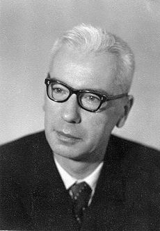
Emile Picard.
The theorem above is usually referred to as Picard's theorem (or sometimes Picard--Lindelöf theorem or the method of successive
approximations) named after Émile Picard (1858--1941) who proved
this result based on iteration procedure. Ernst Leonard Lindelöf (1870--1946) was a Finnish mathematician and Charles Émile Picard was a French
mathematician. Rudolf Otto Sigismund Lipschitz (1832--1903) was a German mathematician who gave his name to the Lipschitz continuity condition.
Picard's mathematical papers, textbooks, and many popular writings exhibit an extraordinary range of interests, as well as an impressive
mastery of the mathematics of his time. In addition to his theoretical work, Picard made contributions to applied mathematics, including the theories
of telegraphy and elasticity. Picard's popular writings include biographies of many leading French mathematicians, including his father in law,
Charles Hermite.
Any differential operator is an unbounded operator. This prevents of using it in well-known fixed point theorems. Fortunately, there is a way to bypass this obstacle by transferring the initial value problem into an integral equation of the second kind. Since an integration is a bounded operation, it allows us to apply the method of successive approximations.
Since the initial value problem \( y' = f(x,y) , \qquad y(x_0 ) = y_0 \) is equivalent to the Volterra integral equation (subject that the slope function f(x,y) and the solution y(x) are continuous functions)
this problem has a unique solution that is the limit of the sequence of
functions \( \left\{ \phi_n (x) \right\}_{n\ge 0} \) that satisfies the recurrence:
Solving this initial value problem is a subject of calculus because the right-hand side is a known function.
However, it is impossible to prove convergence of its solutions because the initial value problem involves the unbounded derivative operator. So we are forced to stick with the Volterra equations \eqref{EqExis.4} in order to prove the convergence of its solutions.
Proof:
Starting with the initial constant function
\( \phi_0 = y_0 , \) successive terms are defined
recursively:
Next we show that our sequence of partial sums for series (Picard.1) converges uniformly to a limit for
| x - x0 | \le; h. Recall that the Weierstrass M-Test assues us that if every function fn(x) is bounded \( \left\vert f_n (x) \right\vert \le M_n for all n ≥ 1 and all x in some interval A, and \( \sum_n M_n \) converges, then the series \( \sum_n f_n (x) \) converges absolutely and uniformly on A.
Therefore,
by the Weierstrass M-Test, we have
Therefore, the sequence of Picard's iteration converges uniformly for all
x from some finite interval
[x0 - h, x0 + h].
The last step is to prove that the limit function φ(x) satisfies the
differential equation \( y' = f(x,y) \) and the
initial condition y(0) = y0.
This follows immediately from equivalence of the initial value problem and the
corresponding Volterra integral equation. Note that the latter statement is
valid only for continuous functions, so requirement that the slope function
f(x,y) is continuous is essential.
▣
Corollary 2:: The continuous dependence of the solutions on the initial conditions holds whenever slope function f satisfies a global Lipschitz condition.
⧫
Corollary 3:: If the solution y(x) of the initial value problem \( y' = f(x,y), \ y(x_0 )= y_0 \) has an a priori bound M, i.e., \( |y(x)| \le M \) whenever y(x) exists, then the solution exists for all \( x \in \mathbb{R} . \)
⧫
Notes:
There are two main drawbacks in application of Picard's iteration scheme. If differential equation is not autonomous (so slope function depends on both, independent and dependent variables), then Picard's iteration always produces some noise terms at every stage. Of course, their contribution is low and next iteration corrects them, but new noise terms appear.
Generally speaking, Picard's iteration method is applicable only to differential equations with polynomial slope functions; otherwise integration cannot be performed explicitly. In tutorial II, it will be shown how this obstacle can be bypassed in many practical cases. Another approach was demonstrated by the brilliant scientist
Lloyd Nicholas Trefethen (born 30 August 1955 in Boston, Massachusetts) who suggested to approximate slope functions with Chebyshev polynomials first and based on their expansions apply Picard's iteration. This numerical method was implemented in the Chebfun package---a clear demonstration how fruitful can be a combination of analytical tools with computational techniques.
Example 2:
Consider the initial value problem for the Riccati equation
\[
y' = x^2 + y^2, \quad y(0)=0 ,
\tag{1.1}
\]
which has a unique solution \( y = \phi (x) \) expressed via Bessel functions
You see that the first term is crrect, but thre second one is not. When determine next Picard's iterative terms, we will put correct terms in bold font so you can observe noise terms.
Therefore, we can make an observation that every next iteration gives a new correct terms along with some other noise terms. Moreover, the number of terms grows as a snow ball---this method cannot be considered as a practical one.
■
Example 3:
Consider the initial value problem for the first order differential equation
If we start with the initial condition ϕ0 = 1, we almost immediately come to a problem of explicit integration. Indeed, we calculate first the few terms:
This example illustrates that Picard's scheme is not practical because the corresponding iteration cannot be performed indefinitely---the functions are not explicitly integrable. In order to apply Picard's method, the slope function must be a polynomial---otherwise the results of integration cannot be expressed through elementary functions.
End of Example 2
■
There are known several improvements and generalizations of Picard's existence theorem. The following one, credited to the famous Russian mathematician Sergei Lozinsky (1914--1985). One substantial advantage of the Lozinsky statement compared to classical Picard's iteration consists in determination of wider domain of existence.
Sergey Lozinsky.
Theorem (Lozinsky): Let f(x,y) be a real-valued continuous function in some domain Ω ⊂ ℝ²
and M(x) be a nonnegative continuous function on some finite
interval \( I \ (x_1 \le x \le x_1 ) \) inside
Ω. Let \( |f(x,y)| \le M(x) \) for x
∈ I and (x,y) ∈ Ω. Suppose that the closed
domain Q, defined by inequalities
\[
x_0 \le x \le x_1 , \qquad
\left\vert y - y_0 \right\vert \le \int_{x_0}^x M(u)\,{\text d}u ,
\]
is a subset of Ω and there exists a nonnegative integrable function
k(x), k ∈ I.such that
\[
\phi_{n+1} (x) = y_0 + \int_{x_0}^x f \left( s, \phi_n (s) \right) {\text d}s
\]
defines the sequence of functions { φn(x) } that
converges to a unique solution of the initial value problem
\( y' = f(x,y), \ y(x_0 ) = y_0 \)
provided that all points (x, φn(x)) are included
in Q when x0 ≤ x ≤ x1.
Moreover,
The theorem above was proved by the famous Russian mathematician
Sergey Mikhailovich Lozinskii/Lozinsky (1914--1985), student of V.I. Smirnov
and S.N. Bernstein. Sergey Lozinsky made many important contributions to the
error estimation methods for various types of approximation solutions of
ordinary differential equations. During two years (1941-1942) he was in active
military duties on defending Leningrad (now St. Petersburg).
Example 4:.
Consider the initial value problem for the Riccati equation
\[
y' = x^2 + y^2, \quad y(0)=0 ,
\]
which has a unique solution \( y = \phi (x) \) expressed via Bessel functions
This function blows up at \( x \approx 2.003147359 \) --- the first positive root of the transcendent equation \( J_{1/4} \left( \frac{x^2}{2} \right) = Y_{1/4} \left( \frac{x^2}{2} \right) . \)
Actually, Picard's theorem guarantees a unique solution within the interval \( \left[ 0, 2^{-1/2} \right] \approx [0,0.707107 ] . \) To find its solution, we use Picard's iteration procedure:
We can extend the Picard domain of existence [0, 0.707] with the aid of the Lozinsky theorem. Let us consider the domain Ω defined by inequalities (containing positive numbers x1 and A to be determined)
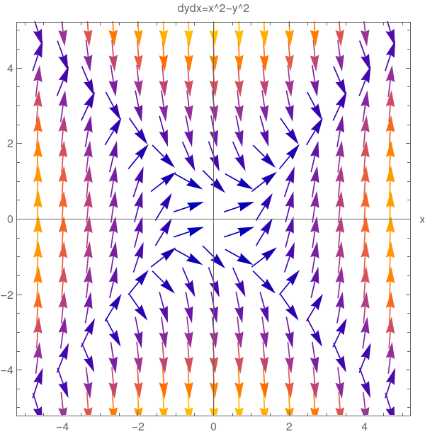
For the function x² −y² in the rectangle |x| ≤ 𝑎, |y| ≤ b, the Picard theorem guarantees the existence of a unique solution within the interval |x| ≤ h. where
\[
h = \min \left\{ a, \ \frac{b}{\max \left\{ a^2 , b^2 \right\}} \right\} \le 1 .
\]
Upon plotting the corresponding direction field, we see that solution of the given initial value problem exists for all x., but Picard's theorem assues us about finite interval,
To extend the interval of existence, we apply the Lozinsky theorem. First, we consider the function x² −y² in the domain Ω bounded by inequalities \( 0 \le x \le x_p^{\ast} \quad \) and \( \quad |y| \le A\,x^p , \quad \) where A and p are some positive constants and \( \quad x_p^{\ast} \quad \) will be determined shortly. Then
In order to guarantee inclusion Q &subset Ω, the following inequality should hold: \( \quad \int_0^x M(u)\,{\text d}u \le A\,x^p . \quad \) It is valid valid in the interval
\( \quad \epsilon < x < x_p^{\ast} , \quad \) where \( x_p^{\ast} \) is the root of the equation
\( \quad \int_0^x M(u)\,{\text d}u = A\,x^p \quad \) and ϵ is a small number.
When A → +0 and p → 1+0, the root
\( x_p^{\ast} \) could be made arbitrary large. For instance, when A = 0.001 and p = 1.001, the root is
\( \quad x_p^{\ast} \approx 54.69. Therefore, the given IVP has a solution on the whole line −∞ < x < ∞.
Coddington, Earl A.; Levinson, Norman (1955). Theory of Ordinary Differential Equations. New York: McGraw-Hill.
Gardner, C., Another elementary proof of Peano existence theorem, The American Mathematical Monthly, 1976
Hsu, S.-B., Ordinary Differential Equations with Applications, Second edition, World Scientific, 2013.
Kennedy, H.C., Is there an elementary proof of Peano's existence theorem for first order differential equations? The American Mathematical Monthly, 1969, Vol. 76, No. 9, pp. 1043--1045.
Murray, F.J. and Miller, K.S., Existence Theorems for Ordinary Differential Equations, Dover Publications; Dover Ed edition (June 5, 2007)
Peano, G., "Sull'integrabilità delle equazioni differenziali del primo ordine". 1886, Atti Accad. Sci. Torino. 21: 437–445.
Teschl, Gerald (2012). Ordinary Differential Equations and Dynamical Systems. Providence: American Mathematical Society. ISBN 978-0-8218-8328-0.
Walter, J., On elementary proofd of Peano's existence theorems,
Return to Mathematica page
Return to the main page (APMA0330)
Return to the Part 1 (Plotting)
Return to the Part 2 (First Order ODEs)
Return to the Part 3 (Numerical Methods)
Return to the Part 4 (Second and Higher Order ODEs)
Return to the Part 5 (Series and Recurrences)
Return to the Part 6 (Laplace Transform)
Return to the Part 7 (Boundary Value Problems)