Preface


Solving equations of the form: \( \frac{{\text d}y}{{\text d}x} = f \left( \frac{ax+by+c}{Ax+By +C} \right) , \quad Ax+By +C \ne 0 \) was first accomplished by Carl Jacobi (1804--1851) in 1842 (Journal für die reine und angewandte Mathematik).

Return to computing page for the first course APMA0330
Return to computing page for the second course APMA0340
Return to Mathematica tutorial for the second course APMA0340
Return to the main page for the course APMA0330
Return to the main page for the course APMA0340
Return to Part II of the course APMA0330

Equations with Linear Fractions


A wide class of differential equations of the form
\[ \frac{{\text d}y}{{\text d}x} = f \left( \frac{ax+by+c}{Ax+By +C} \right) , \qquad Ax+By +C \ne 0, \]
can be reduced to separable equations. Here a, b, c, and A, B, C are some given constants and the function of one variable f(v) is assumed to be continuous within some interval. Without any loss of generality, we consider only the case when two lines defined by equations ax+by+c = 0 and Ax+By+C = 0 are not parallel (\( aB - Ab \ne 0 \) ). Otherwise, the above equation can be reduced to a separable equation upon substitution v = ax+by+c or v = Ax+By+C, which was demonstrated in the previous section.

If \( aB - Ab \ne 0 ,\) constants c and C can be eliminated by shifting the system of coordinates:

\[ x = X + \alpha \quad \mbox{and} \quad y = Y + \beta \qquad\Longrightarrow \qquad X = x- \alpha , \quad Y = y - \beta , \]
with constants α and β to be chosen to satisfy the system of equations:
\[ a\alpha + b\beta + c =0 \qquad \mbox{and} \qquad A\alpha + B \beta +C =0 . \]
With these choices, we get the differential equation in new variables X and Y:
\[ \frac{{\text d}Y}{{\text d}X} = f \left( \frac{aX+bY}{AX+BY} \right) = f \left( \frac{a+bY/X}{A+BY/X} \right) , \qquad AX+BY \ne 1 , \]
which can be reduced to a separable one by substitution v = Y/X.

We start our exposition by considering equations with slope function as the ratio of two linear functions:

Example: : Consider the differential equation:

\[ \frac{{\text d}y}{{\text d}x} = \frac{2x+3y-1}{4x+y-7} , \qquad 4x+y -7 \ne 0. \]
Upon solving system of algebraic equations
\[ 2\alpha + 3\beta -1 =0 \qquad \mbox{and} \qquad 4\alpha + \beta -7 =0 , \]
we find that we need to make substitution:
\[ x = X +2 \quad \mbox{and} \quad y = Y -1 \qquad\Longrightarrow \qquad X = x- 2 , \quad Y = y +1 . \]
With such choice of α = 2 and β = -1, we obtain a differential equation in new variables X and Y, where slope function depends on the ratio v = Y/X:
\[ \frac{{\text d}Y}{{\text d}X} = \frac{2X+3Y}{4X+Y} = \frac{2+3Y/X}{4+Y/X}, \qquad Y \ne -4X. \]
Setting v = Y/X, we get a separable equation
\[ X\,\frac{{\text d}v}{{\text d}X} +v = \frac{2+3v}{4+v} \qquad\Longrightarrow \qquad X\,\frac{{\text d}v}{{\text d}X} = \frac{2+3v}{4+v} -v = - \frac{v^2 +v -2}{4+v} = - \frac{(v +2)(v-1)}{4+v}, \qquad v \ne -4. \]
Upon separation of variables and integration, we obtain
\[ \frac{\left( 4 + v \right) {\text d}v}{(v +2)(v-1)} = -\frac{{\text d}X}{X} \qquad\Longrightarrow \qquad \int \frac{\left( 4 + v \right) {\text d}v}{(v +2)(v-1)} = \frac{5}{3}\,\ln |1-v| - \frac{2}{3}\,\ln |2+v| = - \int \frac{{\text d}X}{X} = - \ln KX = \ln K\,X^{-1} , \]
where K is a constant of integration, and two values v=-2 and v=1 should be excluded because of presence of two logarithms. Previously, we excluded v=-4 from our consideration since the slope function has v+4 in the denominator. Dropping logarithm sign, we get
\[ \frac{|1-v|^5}{(2+v)^2} = \frac{K}{X^3} \qquad\Longrightarrow \qquad X^5 |1-v|^5 = K\,X^2 \, (2+v)^2 , \qquad v \ne -2 . \]
We set back v = Y/X and have
\[ |X-Y|^5 = K \, (2X+Y)^2 , \qquad Y \ne -2X, \quad Y\ne X, \quad Y \ne -4X . \]
In order to obtain the general solution of the given differential equation, we just need to substitute X = x-2 and Y = y+1 into the above relation:
\[ |x-y-3|^5 = K \, (2x+y -3)^2 , \qquad y+2x-3 \ne 0, \quad y-x+3 \ne 0, \quad 4x+y -7 \ne 0 . \]
Finally, we need to check whether excluded functions y = -2x+3 and y = x-3 are solutions of the given differential equation. Indeed they are. Moreover, these two functions can be obtained from the above general solution by appropriate choice of constant K, namely, taking either zero or infinity.

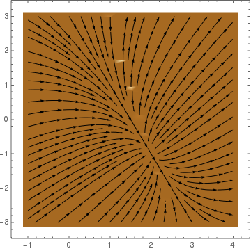
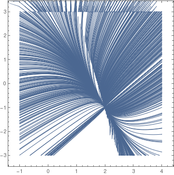
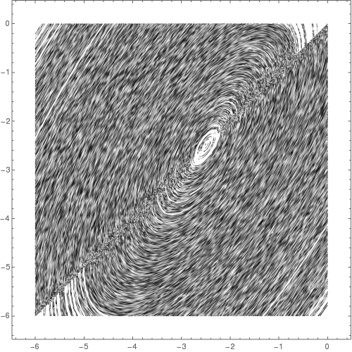
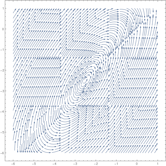
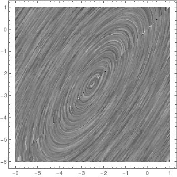
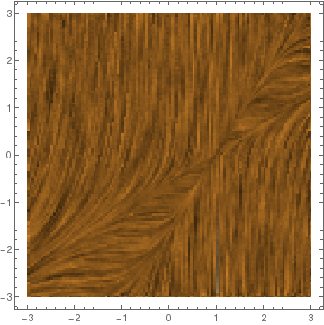
We plot the corresponding direction fields using StreamPlot command:

StreamDensityPlot[{1, (2*x + 3*y - 1)/(4*x + y - 7)}, {x, -1, 4}, {y, -3, 3}, StreamStyle -> Black]
StreamPlot[{1, (2*x + 3*y - 1)/(4*x + y - 7)}, {x, -1, 4}, {y, -3, 3},
StreamPoints -> {Tuples[Range[-1, 4, 0.2], 2], Automatic, 10},
ImageSize -> Medium, StreamStyle -> "Line"]
   

Example: : 
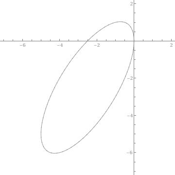
Consider an algebraic equation: \( 2 x^2 + y^2 - 2 x y + 5 x =0 \) and we wish to determine a differential equation to which the algebraic equation defines implicitly its solution. Mathematica is capable to find the required differential equation.

eq = 2 x^2 + y^2 - 2 x y + 5 x == 0
Out[1]= 5 x + 2 x^2 - 2 x y + y^2 == 0

To extract the left-hand side, type:

eq[[1]]
Out[4]= 5 x + 2 x^2 - 2 x y + y^2
Then we plot the graph:
ContourPlot[Evaluate[eq[[1]]], {x, -7, 2}, {y, -7, 2}, Frame -> False,
Axes -> Automatic, AxesOrigin -> {0, 0},
AxesStyle -> GrayLevel[0.5], PlotPoints -> 100, Contours -> {0},
ContourShading -> False]

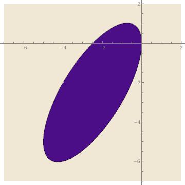
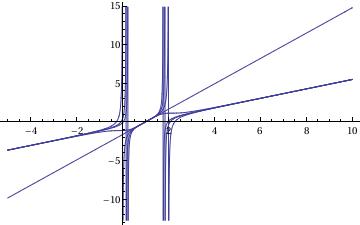
If the option ContourShading is removed, we will get

In the above graphs, the option Contour->{0} instructs Mathematica to graph only the level curve corresponding to 0.
The option ContourShading -> False specifies to not shade the regions between contours,
Frame -> False specifies that a frame is not to be placed around the resulting graphics objects,
Axes -> Automatic specifies that axes are to be placed on the resulting graphics objects while the option
AxesOrigin -> {0, 0} specifies that they intersect at the point (0,0), and the option
AxesStyle -> GrayLevel[0.5] specifies that they be drawn in a medium shade of gray.
The option PlotPoints -> 100 instructs Mathematica to increase the number of sample points to 100 (the default is 15), helping assure that the resulting graphic object appears smooth.
Note that instead of eq[[1]], one can use the equation 5 x + 2 x^2 - 2 x y + y^2 explicitly.

Now we instruct Mathematica to find the differential equation in two steps.

step1= Dt[eq,x]
Out[2]= 5 + 4 x - 2 y - 2 x Dt[y, x] + 2 y Dt[y, x] == 0
step2=Solve[step1,Dt[y,x]]
Out[3]= {{Dt[y, x] -> (5 + 4 x - 2 y)/(2 (x - y))}}

Therefore, we get the differential equation

\[ \frac{{\text d}y}{{\text d}x} = \frac{5 + 4 x - 2 y}{2 (x - y)} , \qquad x\ne y. \]
The plotted direction field confirms that the original algebraic equation defines its solution implicitly.
t = Map[StreamPlot[{1, (5 + 4*x - 2*y)/2/(x - y)}, {x, -6, 0}, {y, -6, 0}, StreamStyle -> "Line",
StreamPoints -> RandomReal[{-6, 0}, {#, 2}],
StreamColorFunction -> (GrayLevel[RandomReal[]] &),
ImageSize -> 500] &, ConstantArray[50, 100]];

Show[t]
f[x_, y_] := {1, (5 + 4*x - 2*y)/2/(x - y)};
xrange = {-6, 1};
yrange = {-6, 1};
xdivs = 3;
ydivs = 3;
xranges = Partition[Rescale[Range[0, xdivs], {0, xdivs}, xrange], 2, 1];
yranges = Partition[Rescale[Range[0, ydivs], {0, ydivs}, yrange], 2, 1];

Show[Flatten@
Table[StreamPlot[
f[x, y], {x, First@xr, Last@xr}, {y, First@yr, Last@yr},
StreamScale -> {0.2, Automatic, 0.01}, StreamPoints -> 100], {xr,
xranges}, {yr, yranges}], PlotRange -> All, ImageSize -> Large]
LineIntegralConvolutionPlot[{1, (5 + 4*x - 2*y)/2/(x - y)}, {x, -6, 1}, {y, -6, 1},
LineIntegralConvolutionScale -> 0.6,
ColorFunction -> GrayLevel, RasterSize -> 200]
     

Example: : Consider the differential equation

\[ \frac{{\text d}y}{{\text d}x} = \frac{(2x-2y-2)^2}{(x-1)^2} , \qquad x \ne 1. \]
We exclude the singular point x = 1 where the integral curves have an infinite slope. The right-hand side function (= slope function) is a composition of two functions:
\[ \frac{(2x-2y-2)^2}{(x-1)^2} = F(z(x,y)) , \qquad\mbox{where} \quad F(z) = z^2 \quad \mbox{and} \quad z = (2x-2y-2) / (x-1) . \]
The function F(z(x,y)) is not homogeneous, but it can be converted to a homogeneous one by shifting
\[ x=X+\alpha \qquad \mbox{and}\qquad y=Y+\beta , \]
where \( \alpha = 1, \) and \( \beta = 0 ,\) so \( x=X+1, \ y=Y.\) We next substitute \( x=X+1 \) and \( y=Y \) into the given differential equation and simplify. The result is
\[ \text{d}Y/\text{d}X = \text{d}y / \text{d}(x-1) = \text{d}y /\text{d}x = (2(x-1) -2y/{x-1} )^2 = ( (2X -2Y) / X )^2 . \]
Setting \( Y=vX \) gives us
\[ X \text{d}v /\text{d}X +v = 4 (1-v)^2 \qquad \mbox{or} \qquad \text{d}v (4(1-v)^2 -v) = \text{d}X / X . \]
Plotting the direction field, it can be seen that \( v = a /2 \approx 1.64039 \) is an unstable equilibrium solution, and \( v= \frac{b}{2} \approx 0.609612 \) is a stable equilibrium solution. These critical points are not singular solutions because integral curves do not touch them, which means that an initial value problem for the differential equation \( X\,v' = (2v-a)(2v-b) \) has a unique solution.

Now we return to the original variables. Since \( X=x-1, \ Y=y \), and \( v=Y/X, \) the original differential equation has the general solution
in implicit form:

\[ C|x-1|^{\sqrt{17}} = \left| \frac{8y -(9 + \sqrt{17})(x-1)}{8y -(9 -\sqrt{17})(x-1)} \right| , \qquad x \ne 1. \]
It can be solved with respect to y, and then plotted using the following Mathematica commands:
a:=Abs[Sqrt[17]];
Plot[((x - 1)*(#1 Abs[x - 1]^a *(9 - a) - 9 - a)/(#1 Abs[x - 1]^a - 1)/ 8 &) /@ {-1, 0, 1, 2, 3}, {x, -5, 10}]
LineIntegralConvolutionPlot[{1, (2*x - 2*y - 2)^2 /(x - 1)^2}, {x, -3, 3}, {y, -3, 3}]
   
The given differential equation has two equilibrium (but not singular) solutions that correspond to v=a/2 and v=b/2:
\[ y = (x-1) a/2 = (x-1)\, \frac{9+\sqrt{17}}{8} \qquad \mbox{and} \qquad y = (x-1) b/2 = (x-1) \, \frac{9-\sqrt{17}}{8} . \]


Return to Mathematica page
Return to the main page (APMA0330)
Return to the Part 1 (Plotting)
Return to the Part 2 (First Order ODEs)
Return to the Part 3 (Numerical Methods)
Return to the Part 4 (Second and Higher Order ODEs)
Return to the Part 5 (Series and Recurrences)
Return to the Part 6 (Laplace Transform)
Return to the Part 7 (Boundary Value Problems)