Return to computing page for the second course APMA0340
Return to Mathematica tutorial for the second course APMA0340
Return to the main page for the course APMA0330
Return to the main page for the course APMA0340
Return to Part IV of the course APMA0330
Glossary
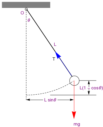
Simple Pendulum
The motion of the pendulum is, evidently, completely characterized by the variable θ, measured in counterclockwise direction as positive. We call θ the generalized coordinate for this system. It arises because the motion is constrained by \( x^2 + y^2 = \ell^2 . \) Even though the pendulum swings in 3 dimensional space, its motion is characterized by a single variable. We say in this case that the pendulum has “one degree of freedom.”
|
polygon = Polygon[{{-1, 0}, {1, 0}, {1, 1/4}, {-1, 1/4}}];
top = Graphics[{Gray, polygon}]; circle1 = Graphics[Circle[{0, -1/20}, 1/20]]; circle2 = Graphics[Circle[{2, -3}, 1/5]]; circle3 = Graphics[{Dashed, Circle[{0, 0}, 3.6, {-1.57, -1.0}]}]; line1 = Graphics[{Dashed, Line[{{0, -1/20}, {0, -3.8}}]}]; line2 = Graphics[{Thick, Line[{{0.03, -0.07}, {1.9, -2.83}}]}]; arrow = Graphics[{Red, Arrowheads[0.08], Arrow[{{1.986, -3.0}, {1.986, -4.6}}]}]; line3 = Graphics[{Line[{{2.2, -3.8}, {2.9, -3.8}}]}]; arrow2a = Graphics[{Arrowheads[0.04], Arrow[{{0.7, -3.8}, {0, -3.8}}]}]; arrow2b = Graphics[{Arrowheads[0.04], Arrow[{{1.3, -3.8}, {1.98, -3.8}}]}]; text1 = Graphics[ Text[Style["L sin\[Theta]", FontSize -> 14, Purple], {1.0, -3.8}]]; text2 = Graphics[ Text[Style["mg", FontSize -> 14, Purple], {2.1, -4.8}]]; line3 = Graphics[{Line[{{1.0, -3.6}, {2.9, -3.6}}]}]; line4 = Graphics[{Line[{{2.2, -3.0}, {2.9, -3.0}}]}]; text3 = Graphics[ Text[Style["L(1 - cos\[Theta])", FontSize -> 14, Purple], {2.7, -3.3}]]; arrow3a = Graphics[{Arrowheads[0.04], Arrow[{{2.6, -3.35}, {2.6, -3.6}}]}]; arrow3b = Graphics[{Arrowheads[0.04], Arrow[{{2.6, -3.27}, {2.6, -3.0}}]}]; text4 = Graphics[ Text[Style["L", FontSize -> 14, Purple], {1.2, -1.5}]]; text5 = Graphics[ Text[Style["\[Theta]", FontSize -> 14, Purple], {0.1, -0.5}]]; text6 = Graphics[ Text[Style["O", FontSize -> 14, Purple], {-0.16, -0.2}]]; textT = Graphics[ Text[Style["T", FontSize -> 14, Black], {1.15, -2.1}]]; arrowT = Graphics[{Blue, Arrowheads[0.08], Arrow[{{1.88, -2.8}, {1.2, -1.8}}]}]; Show[top, circle1, circle2, circle3, line1, line2, line3, arrow, arrow2a, arrow2b, text1, text2, line4, text3, arrow3a, arrow3b, text4, text5, text6, arrowT, textT] |
 |
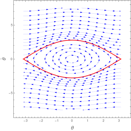
There are known two general approaches to derive the pendulum equation. The first one is based on Newton's second law (written for rotational motion):
Show[StreamPlot[{y, -9.81/l Sin[x]}, {x, - Pi, Pi}, {y, -7.5, 7.5}, FrameLabel -> {Style["\[Theta]", 16], Style["\!\(\*OverscriptBox[\(\[Theta]\), \(.\)]\)", 16]}, StreamPoints -> 50, StreamStyle -> {Blue, Thin}],
ContourPlot[ y^2/2 - 9.81/l Cos[x] == 9.81/l, {x, - Pi, Pi}, {y, -7.5, 7.5},
ContourStyle -> {Thick, Red}], ImageSize -> 1.1 {400, 400}], {{l, 4, "pendulum length"}, 1, 10, 0.1, Appearance -> "Labeled"}]
The second approach is based on the Euler--Lagrange equation (which we formulate for one degree of freedom, in our case):
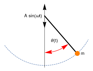
Example: Consider a simple pendulum problem when its pivot is undergoing vertical oscillations given by A sin(ωt) as shown. To solve this parametric excitation problem, the rectangular coordinates of the mass m are first expressed in terms of the length ℓ and angle θ(t), t being time.
 |
a = {Graphics[{Arrowheads[{-0.07, 0.07}],
Arrow[{{0, -0.5}, {0, 0.5}}]}]};
dash = ParametricPlot[{2.02*Cos[t], 2.02*Sin[t]}, {t, -2.5, -0.5}, PlotStyle -> Dashed, Axes -> False]; vline = Graphics[Line[{{0, 0}, {0, -2.1}}]]; angle = ParametricPlot[#[[1]]*{Cos[\[Theta]], Sin[\[Theta]]}, {\[Theta], #[[2]], #[[3]]}, Axes -> False, PlotStyle -> #[[4]]] /. Line[x_] :> Sequence[Arrowheads[{-0.08, 0.08}], Arrow[x]] & /@ {{-1.5, 90 Degree, 130 Degree, Red}}; line = Graphics[{Thickness[0.01], Line[{{0, 0}, {1.25, -1.45}}]}]; disk = Graphics[{Orange, Disk[{1.33, -1.53}, 0.1]}]; sin = Graphics[ Text[Style["A sin(\[Omega]t)", FontSize -> 16, Black], {-0.46, 0.0}]]; theta = Graphics[ Text[Style["\[Theta](t)", FontSize -> 16, Black], {0.4, -1.0}]]; m = Graphics[Text[Style["m", FontSize -> 16, Black], {1.55, -1.53}]]; Show[dash, a, vline, angle, line, disk, sin, m, theta, PlotRange -> All] |
Simplify command, we get
Example: Consider a pendulum excited both at a slow and a high frequency. The motion of the pendulum is governed by the following equation: ̈
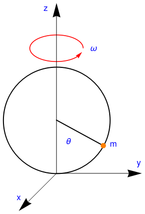
Example: A vertically oriented circular wire of radius ℓ rotates with angular velocity ω about the z-axis. A bead of unit mass (m = 1) is allowed to slide along the frictionless wire.
 |
arc = Show[
ParametricPlot[#[[1]]*{Cos[\[Theta]]*0.5 - 1.35,
0.25 Sin[\[Theta]]} + 1.35, {\[Theta], #[[2]], #[[3]]},
Axes -> False, PlotStyle -> #[[4]]] /.
Line[x_] :> Sequence[Arrowheads[{0, 0.05}], Arrow[x]] & /@ {{1,
0 , 6, Red}}, PlotRange -> All]
circle = Graphics[{Thick, Circle[{0, 0}, 1]}] arrowx = Graphics[{Arrowheads[0.1], Arrow[{{0, -1}, {-0.707, -1.707}}]}] arrowy = Graphics[{Arrowheads[0.1], Arrow[{{0, -1}, {1.6, -1}}]}] arrowz = Graphics[{Arrowheads[0.1], Arrow[{{0, -1}, {0, 2.2}}]}] line = Graphics[{Thick, Line[{{0, 0}, {0.877, -0.479}}]}] disk = Graphics[{Orange, Disk[{0.877, -0.479}, 0.05]}] txtx = Graphics[Text[Style["x", FontSize -> 16, Blue], {-0.7, -1.45}]] txty = Graphics[Text[Style["y", FontSize -> 16, Blue], {1.55, -0.8}]] txtz = Graphics[Text[Style["z", FontSize -> 16, Blue], {-0.2, 2.1}]] txto = Graphics[ Text[Style["\[Omega]", FontSize -> 16, Blue], {0.7, 1.35}]] txtt = Graphics[ Text[Style["\[Theta]", FontSize -> 16, Blue], {0.23, -0.4}]] txtm = Graphics[Text[Style["m", FontSize -> 16, Blue], {1.07, -0.45}]] Show[circle, arc, arrowx, arrowy, arrowz, line, disk, txtx, txty, \ txtz, txto, txtt, txtm] |
Plot[Evaluate[y[t] /. ssol], {t, 0, 20}, PlotPoints -> 1000, Frame -> True, PlotStyle -> {Thick, Hue[0.9]}, FrameLabel -> {"time", "angle"}, ImageSize -> {600, 400}, LabelStyle -> {FontFamily -> "Times", FontSize -> 16}]
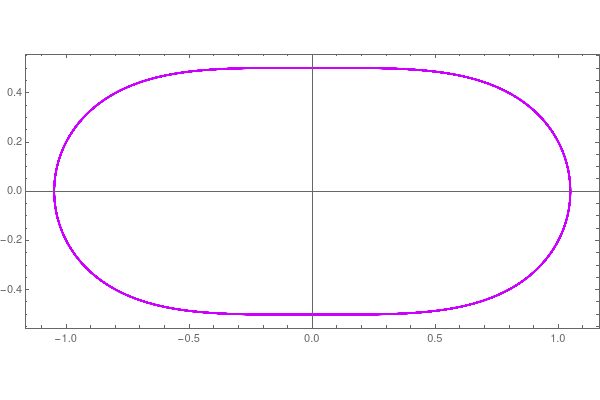
ParametricPlot[ Evaluate[{y[t], y'[t]} /. ssol, {t, 0, 100}, Frame -> True, PlotStyle -> Hue[0.8], ImageSize -> {600, 400}]]
 |
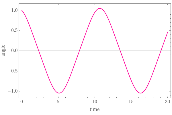 |
| Graph of angle vs time | Graph of angle vs velocity |
- Scientific Computing by Jeffrey R. Chasnov.
- Fidlin, A., Bi-harmonically excited pendulum: shifted resonances and quenching the low frequency excitation, 2006, PAMM Proc Appl Math Mech , Volume 6, pp. 301--302. doi: 10.1002/pamm.200610132
- Fidlin, A., Nonlinear Oscillations in Mechanical Engineering, 2006, Springer-Verlag, Berlin, New York.
- Ganji, D.D., Karimpour, S., and Ganji, S.S., Approximate analytical solutions to nonlinear oscilations of non-natural systems using He's energy balance method, Progress in Electromagnetics Research, 2008, Vol. 5, pp. 43--54.
Return to Mathematica page
Return to the main page (APMA0330)
Return to the Part 1 (Plotting)
Return to the Part 2 (First Order ODEs)
Return to the Part 3 (Numerical Methods)
Return to the Part 4 (Second and Higher Order ODEs)
Return to the Part 5 (Series and Recurrences)
Return to the Part 6 (Laplace Transform)
Return to the Part 7 (Boundary Value Problems)