Preface
This section demonstrates an application of the power series method in solving first order differential equations.
Return to computing page for the second course APMA0340
Return to Mathematica tutorial for the second course APMA0340
Return to the main page for the course APMA0330
Return to the main page for the course APMA0340
Return to Part V of the course APMA0330
Glossary
Examples for first order ODEs solved by Power Series
We believe that the best way to learn a material and techniques is go by examples. Therefore, this section contains a detail exposition of several examples.
Example: Consider the initial value problem
Example: Consider the initial value problem
ProductLog is another name for Lambert function.
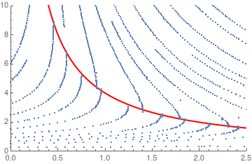
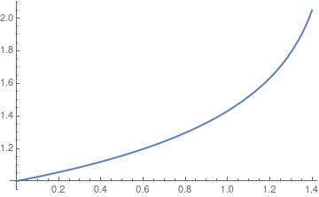
Then we plot its solution using standard Mathematica command
NDSolve and display the corresponding stream plot along with
the singular line (in red) y = 4/x.
Plot[y[x] /. sol, {x, 0, 1.4}, PlotStyle -> Thick]
stream = ListPlot[ Reap[StreamPlot[{1, y^2/(4 - x*y)}, {x, 0, 2.5}, {y, 0, 10}, EvaluationMonitor :> Sow[{x, y}]]][[-1, 1]]]
hyper = Plot[4/x, {x, 0.3, 2.6}, PlotStyle -> {Thick, Red}, PlotRange -> {{0, 2.5}, {0, 10}}]
Show[hyper, stream]
|
|
| Stream plot | Solution curve |
The given differential equation has a moving singularity: y = 4/x, indicated on the graph by red curve. Now we seek its solution in power series form:
Example: Consider the initial value problem
- Duan, J.-S. and Rach, R., The degenerate form of the Adomian polynomials in the power series method for nonlinear ordinary differential equations, Journal of Mathematics and System Science, Volume 5, Pages 411--428, doi: 10.17265/2159-5291/2015.10.003
Return to Mathematica page
Return to the main page (APMA0330)
Return to the Part 1 (Plotting)
Return to the Part 2 (First Order ODEs)
Return to the Part 3 (Numerical Methods)
Return to the Part 4 (Second and Higher Order ODEs)
Return to the Part 5 (Series and Recurrences)
Return to the Part 6 (Laplace Transform)
Return to the Part 7 (Boundary Value Problems)