Preface
This chapter gives an introduction to numerical methods used in solving ordinary differential equations of first order. Its purpose is not to give a comprehensive treatment of this huge topic, but to acquaint the reader with the basic ideas and techniques used in numerical solutions of differential equations. It also tries to dissolve a myth that Mathematica is not suitable for numerical calculations with numerous examples where iteration is an essential part of algorithms.
Return to computing page for the second course APMA0340
Return to Mathematica tutorial for the first course APMA0330
Return to Mathematica tutorial for the second course APMA0340
Return to the main page for the course APMA0330
Return to the main page for the course APMA0340
Return to Part III of the course APMA0330
Glossary
RC&RL circuits
The fundamental passive linear circuit elements are the resistor (R), capacitor (C) and inductor (L) or coil. These circuit elements can be combined to form an electrical circuit in four distinct ways: the RC circuit, the RL circuit, the LC circuit and the RLC circuit with the abbreviations indicating which components are used. RC and RL are one of the most basics examples of electric circuits and yet they are very rich in content. The manner in which voltage or current varies with time is referred as time response. We are going to determine currents and voltages that arise when energy is either acquired or released by an inductor or capacitor in response to a change in a voltage or current source.
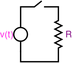
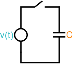
We consider first the response of the three basic idealized passive circuit elements (resistance, inductance, and capacitance) to a steady state sinusoidal excitation.
 |
 |
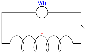 |
| Resistance | Capacitance | Inductance |
The voltage v across a capacitor is related to the electric charge q by v = Sq, where S = 1/C is the elastance, the inverse of capacitance. The terms elastance and elastivity were coined by Oliver Heaviside in 1886. Since the current is i = dq/dt, an integration gives
An inductor, also called a coil, choke, or reactor, is a passive two-terminal electrical component that stores energy in a magnetic field when electric current flows through it. Any change in the current through an inductor creates a changing flux, inducing a voltage across the inductor. By Faraday's law of induction, the voltage induced by any change in magnetic flux through the circuit is given by
Resistance is the capacity of materials to impede the flow of current or, more specifically, the flow of electric charge. The circuit element used to model this behavior is the resistor. Most materials exhibit measurable resistance to current. The amount of resistance depends on the material. Metals such as copper and aluminum have small values of resistance, making them good choices for wiring used to conduct electric current. In fact, when represented in a circuit diagram, copper or aluminum wiring isn;t usually modeled as a resistor: the resistance of the wire is so small compared to the resistance of other elements in the circuit that we can neglect the wiring resistance to simplify the diagram.
For purposes of current analysis, we must reference the current in the resistor to the terminal voltage, We can do so in two ways: either jn the durection of the voltage drop across the resistor or in the direction of the voltage rise across the resistor. If we choose the former, the relatuinship between the voltage and current is
Sinusoidal voltage applied
Suppose that each isolated pure circuit elements R, C, and L, is subject to applied sinusoidal voltage given by
Sinusoidal current applied
Suppose that each isolated pure circuit elements R, C, and L, is subject to applied sinusoidal current given by
Real circuits
In practice, lumped circuit elements designed to behave as pure resistances, inductances, and capacitances must inherently have some combination of all three properties. Since inductance and capacitance depend essentially on the geometry of the element, it is possible to design elements in which these parameters are negligibly small. Resistance, however, is the one parameter which is difficult to eliminate in inductors and capacitors since it is an inherent property of their constituent elements. Therefore, inductors and capacitors are usually come with a combination with resistors.
The major difference between RC and RL circuits is that the RC circuit stores energy in the form of the electric field while the RL circuit stores energy in the form of magnetic field. Another significant difference between RC and RL circuits is that RC circuit initially offers zero resistance to the current flowing through it and when the capacitor is fully charged, it offers infinite resistance to the current. While the RL circuit initially opposes the current flowing through it but when the steady state is reached it offers zero resistance to the current across the coil. Let’s examine each one carefully. Since the voltages and currents of the basic RL and RC circuits are described by first order differential equations, these basic RL and RC circuits are called the first order circuits.
RC circuits
Suppose that we wish to analyze how an electric current flows through a circuit. An RC circuit is a very simple circuit might contain a voltage source, a capacitor, and a resistor (see Figure). A battery or generator is an example of a voltage source. The glowing red heating element in a toaster or an electric stove is an example of something that provides resistance in a circuit. A capacitor stores an electrical charge and can be made by separating two metal plates with an insulating material. Capacitors are used to power the electronic flashes for cameras. Current, I(t), is the rate at which a charge flows through this circuit and is measured in amperes or amps (A). We assign a direction to the current. A current flowing in the opposite direction will be given negative values.
Line[{{-4, 0}, {0, 0}, {0.5, 1}, {1.5, -1}, {2, 1}, {3, -1}, {3.5, 1},
{4.5, -1}, {5, 1}, {6, -1}, {6.5, 1}, {7.5, -1}, {8, 0}, {12, 0}}], Axes -> False]
line1 = ListLinePlot[{{-4, 0}, {-4, -3}}, Axes -> False]
line2 = ListLinePlot[{{12, 0}, {12, -3}}, Axes -> False]
line3 = ListLinePlot[{{11.5, -4}, {12.5, -4}}, Axes -> False]
line4 = ListLinePlot[{{11.5, -4.3}, {12.5, -4.3}}, Axes -> False]
line5 = ListLinePlot[{{-4, -5}, {-4, -7}, {12, -7}, {12, -4.3}}, Axes -> False]
c = Graphics[Circle[{-4, -4}, 1]]
Show[res, line1, line2, line3, line4, line5, c]
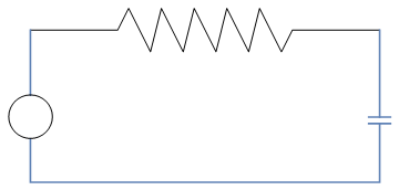
The source voltage, E(t), is measured in volts (V). Kirchhoff's Second Law tells us that the impressed voltage in a closed circuit is equal to the sum of the voltage drops in the rest of the circuit. Thus, we need only compute the voltage drop across the resistor, ER, and the voltage drop across the capacitor, EC. According to Kirchhoff's Law, this is
We will now investigate how our circuit reacts under different voltage sources. For example, we might have a zero voltage source (the capacitor could still hold a charge). We could also have a constant nonzero source of voltage such as a battery or a fluctuating source of voltage such as a generator. We might even have a series of pulses of voltage where the current is periodically turned on and off. We would like to be able to understand the solutions to the above differential equation for different voltage sources E(t). If we view the differential equation as an expression for computing how fast current is flowing across the capacitor, we can analyze our circuit from a geometric point of view and can actually say a great deal about circuits without solving a differential equation.
Example 1: We consider a simplest case when there is no voltage source in the circuit. In this case, the equation
Example 2: If we assume that we have a nonzero constant source of voltage, E(t) = K, in our circuit such as a battery, then we obtain the separable differential equation
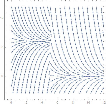
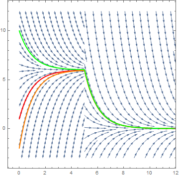
Example 3: If we attach a battery to our circuit at time t = 0 and then disconnect the battery at t = 5, then we obtain a piecewise continuous voltage function. For example, if
st5 = StreamPlot[{1, -y}, {t, 5, 12}, {y, -3, 12}, PlotRange -> {{Full, {5, 12}}, Full}]
Show[st, st5]
s1 = NDSolve[{y'[t] + y[t] == EC[t], y[0] == 1}, y, {t, 0, 30}]
p1 = Plot[Evaluate[y[t] /. s1], {t, 0, 20}, PlotStyle -> {Thick, Red}]
s2 = NDSolve[{y'[t] + y[t] == EC[t], y[0] == -2}, y, {t, 0, 30}]
p2 = Plot[Evaluate[y[t] /. s2], {t, 0, 20}, PlotStyle -> {Thick, Orange}]
s3 = NDSolve[{y'[t] + y[t] == EC[t], y[0] == 10}, y, {t, 0, 30}]
p3 = Plot[Evaluate[y[t] /. s3], {t, 0, 20}, PlotStyle -> {Thick, Green}]
Show[st, st5, p1, p2, p3]
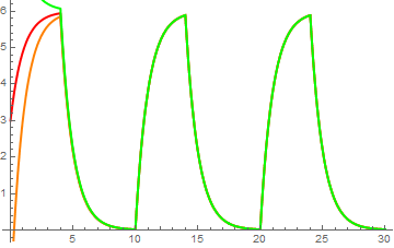
Example 4: Suppose our voltage source emits a series of pulses, say
s1 = NDSolve[{y'[t] + y[t] == EC[t], y[0] == 3}, y, {t, 0, 30}]
p1 = Plot[Evaluate[y[t] /. s1], {t, 0, 30}, PlotStyle -> {Thick, Red}]
s2 = NDSolve[{y'[t] + y[t] == EC[t], y[0] == -2}, y, {t, 0, 30}]
p2 = Plot[Evaluate[y[t] /. s2], {t, 0, 30}, PlotStyle -> {Thick, Orange}]
s3 = NDSolve[{y'[t] + y[t] == EC[t], y[0] == 10}, y, {t, 0, 30}]
p3 = Plot[Evaluate[y[t] /. s3], {t, 0, 30}, PlotStyle -> {Thick, Green}]
Show[p1, p2, p3]
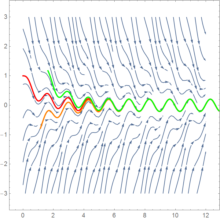
Example: Finally, we consider a generator for a voltage source that might be given by a function such as \( E(t) = \cos \left( 3\pi /2 \right) . \) The direction field for this circuit is given in Figure:
p1 = Plot[Evaluate[y[t] /. s1], {t, 0, 15}, PlotStyle -> {Thick, Red}]
s2 = NDSolve[{y'[t] + y[t] == Cos[3*Pi*t/2], y[0] == -2}, y, {t, 0, 15}]
p2 = Plot[Evaluate[y[t] /. s2], {t, 0, 15}, PlotStyle -> {Thick, Orange}]
s3 = NDSolve[{y'[t] + y[t] == Cos[3*Pi*t/2], y[0] == 5}, y, {t, 0, 15}]
p3 = Plot[Evaluate[y[t] /. s3], {t, 0, 15}, PlotStyle -> {Thick, Green}]
Show[st, p1, p2, p3]
RL circuits
A resistor–inductor circuit (or RL circuit for short) is a circuit that consists of a series combination of resistance and inductance. Energy is stored in the magnetic field generated by a current flowing through the inductor. The induced emf opposes the flow of the current through it. RL circuit contains an inductor, which creates hysteresis and noise in the circuit. Since inductors are large in size, the corresponding RL circuits are bulky and expensive. They are appropriate for filtering of high power signals because of low power dissipation.
An inductor or coil represents the ‘electrical inertia’ of the circuit. As currents flows into the circuit, it generates a magnetic field, that change in the magnetic field causes a change in the flux of the field concatenated to the circuit, this in turn, by the Faraday-Neumann-Lenz law generates a voltage in the circuit that is opposite to the voltage that is generating the magnetic field. As a result, the current in the circuit will not immediately jump to its full value of V/R given by Ohm’s law. What we would expect is that the current will obey the following differential equation given by Ohm’s law at each point in time:
Conclusions
Both equations for RL and RC circuits have the same structure (linear first order differential equation with constant coefficients):
The general solution to the linear differential equation \( \tau\,\dot{y} + y(t) = f(t) \) can be splitted into the sum \( y(t) = y_h (t) + y_p (t) , \) where yh is the general solution of the associated homogeneous equation \( \tau\,\dot{y} + y(t) = 0 \) that does not depend on the driving (excitation) source, and yp is a particular solution or the forced response of the original nonhomogeneous equation. At first glance it may seem odd to expect the current to produce a non zero response with a zero forcing source; however, this behavior stems from the ability of capacitors and inductors to store energy. This voltages and currents will persist until all the initial energy has been used by the resistance in the circuit. Since the homogeneous equation can be written as
In circuit applications, the most special interest is to study the driving responses when forcing function is either DC (= Direct Current = constant value sources) and AC (= Alternated Current = sinusoidal sources) applied suddenly to the circuit. The general solution can be found from the formula:
- Electric Circuits RC and RL
- RL Circuits Lumen Physics
- LR Series Circuit
- RL natural response Khan Academy.
- RL Circuits
- RL Series Circuit
- Natural Response of First Order RC and RL Circuits Mark Whiteley, 2002.
- RL Circuits Libre Texts in Physics.
- First order RL and RC circuitsDallas.
- Zaky, A.A. and Lisboa, C., Response of ideal circuit elements to sinusoidal excitations, American Journal of Physics, 1970, Vol. 38, pp. 1173--1176; http://doi.org/10.1119/1.1975992
Return to Mathematica page
Return to the main page (APMA0330)
Return to the Part 1 (Plotting)
Return to the Part 2 (First Order ODEs)
Return to the Part 3 (Numerical Methods)
Return to the Part 4 (Second and Higher Order ODEs)
Return to the Part 5 (Series and Recurrences)
Return to the Part 6 (Laplace Transform)
Return to the Part 7 (Boundary Value Problems)