Preface
This section is devoted to applications of the modified decomposition method (MDM for short) to the second order differential equations.
Return to computing page for the second course APMA0340
Return to Mathematica tutorial for the first course APMA0330
Return to Mathematica tutorial for the second course APMA0340
Return to the main page for the course APMA0330
Return to the main page for the course APMA0340
Glossary
Modified Decomposition Method 2
The modified decomposition method can be extended for higher order differential equations. We consider the initial values problems for the following second order differential equation \begin{equation} y'' + a(x)\, y + b(x)\, y' = g(x) + f(y) , \qquad y\left( x_0 \right) = \alpha , \quad y'\left( x_0 \right) = \beta , \label{Eadm.8} \end{equation} where 𝑎(x), b(x), and g(x) are holomorphic functions (in applications, these functiosn are usually polynomails) in some neighborhood of the initial point x0, but f(y) is a holomorphoc function in some open domain including points α and β. It is assumed that we know Taylor series expansions of the former functions: \begin{align*} a(x) = \sum_{n\ge 0} a_n \left( x - x_0 \right)^n , \\ b(x) = \sum_{n\ge 0} b_n \left( x - x_0 \right)^n , \\ g(x) = \sum_{n\ge 0} g_n \left( x - x_0 \right)^n . \end{align*} The solution to the initial value problem \eqref{Eadm.8} is asuumed to be represented by a convergent power series \begin{equation} y(x) = \sum_{n\ge 0} u_n (x) = c_0 + c_1 \left( x - x_0 \right) + \sum_{n\ge 2} c_n \left( x - x_0 \right)^n , \qquad c_0 = \alpha , \quad c_1 = \beta . \label{Eadm.1} \end{equation} For application of the modified decomposition method, we also need to know the expansion of the nonlinearity f(y) into the Adomian--Rach series: \[ f(y) = \sum_{n\ge 0} A_n \left( u_0 , u_1 , \ldots , u_n \right) = \sum_{n\ge 0} A_n \left( c_0 , c_1 , \ldots , c_n \right) \left( x - x_0 \right)^n , \] where the Adomian polynomials depend on the components of the solution series \eqref{Eadm.1}. Substituting each power series into the given differential equation and using the convolution formula, we obtain \begin{align*} &\sum_{n\ge 0} \left( n+2 \right) \left( n+1 \right) c_{n+2} \left( x - x_0 \right)^n + \sum_{n\ge 0} \left( a \ast y \right)_n \left( x - x_0 \right)^n + \sum_{n\ge 0} \left( b \ast y' \right)_n \left( x - x_0 \right)^n \\ &= \sum_{n\ge 0} g_n \left( x - x_0 \right)^n + \sum_{n\ge 0} A_n \left( x - x_0 \right)^n \end{align*} where \[ \left( a \ast y \right)_n = \sum_{k=0}^n a_{n-k} c_k \] is the n-component of the convolution of two series (as a result of multiplication of two series). Matching the coefficients of these series, we derive the full-history recurrence \begin{equation} \left( n+2 \right) \left( n+1 \right) c_{n+2} + \sum_{k=0}^n a_{n-k} c_k + \sum_{k=0}^n b_{n-k} c_{k+1} \left( k+1 \right) = g_n + A_n , \qquad n=0,1,2,\ldots . \label{Eadm.10} \end{equation} The initial two terms must be chosen in accordance to the given initial conditions \[ c_0 = \alpha , \qquad c_1 = \beta . \] We demonstrate this technique in the following examples.
Example: The Gross–Pitaevskii equation (GPE, named after Eugene P. Gross and Lev Petrovich Pitaevskii) describes the ground state of a quantum system of identical bosons using the Hartree–Fock approximation and the pseudopotential interaction model. Its simplified stationary version is read as
We first compute the Adomian polynomails for noninear part f(y) = y³:
Example: Consider the initial value problem for the nonlinear differential equation
Example: Consider the initial value problem for the Lane--Emden equation
|
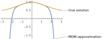
phi5[t_]= 1- t^2/6 + t^4/24 -(5 t^6)/432 + (35 t^8)/10368 - 7* t^(10)/6912;
y[t_]= (1+t^2 /3)^(-1/2); Plot[{phi5[t], y[t]}, {t, -3, 3}, PlotRange -> {-1.2, 1.1}, PlotStyle -> Thick, PlotLabels -> {"MDM-approximation", "true solution"}] |
|
| MDM approximation and the true solution. | Mathematica code |
■
Example: In astrophysics, the Emden–Chandrasekhar equation is a dimensionless form of the Poisson equation for the density distribution of a spherically symmetric isothermal gas sphere subjected to its own gravitational force, named after Robert Emden (1862--1940) and Subrahmanyan Chandrasekhar (1910--1995). The equation was first introduced by Robert Emden in 1907. The equation reads
The Lane--Emden operator admits a factorization:
Ado[5]
For[n = 1, n <= M, n++, c[n, 1] = u[n];
For[k = 2, k <= n, k++, c[n, k] = Expand[1/n* Sum[(j + 1)*u[j + 1]*c[n - 1 - j, k - 1], {j, 0, n - k}]]];
der = Table[D[f[u[0]], {u[0], k}], {k, 1, M}];
A[n] = Take[der, n].Table[c[n, k], {k, 1, n}]]; Table[A[n], {n, 0, M}]]
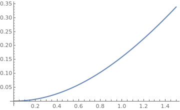
Plot[phi5[x], {x,0,2}, PlotStyle->Thick]
Example: Let us consider the pendulum equation
|
\[
\ddot{\theta} + \omega^2 \sin \theta = 0, \qquad \theta (0) = \theta_0 = \frac{\pi}{3} , \quad \dot{\theta} (0) = 0.
\]
a = {Graphics[{Arrowheads[{0.0, 0.07}],
Arrow[{{0, -0.5}, {0, 0.5}}]}]};
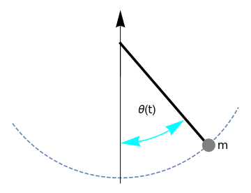
dash = ParametricPlot[{2.02*Cos[t], 2.02*Sin[t]}, {t, -2.5, -0.5}, PlotStyle -> Dashed, Axes -> False]; vline = Graphics[Line[{{0, 0}, {0, -2.1}}]]; angle = ParametricPlot[#[[1]]*{Cos[\[Theta]], Sin[\[Theta]]}, {\[Theta], #[[ 2]], #[[3]]}, Axes -> False, PlotStyle -> #[[4]]] /. Line[x_] :> Sequence[Arrowheads[{-0.08, 0.08}], Arrow[x]] & /@ {{-1.5, 90 Degree, 130 Degree, Cyan}}; line = Graphics[{Thickness[0.01], Line[{{0, 0}, {1.25, -1.45}}]}]; disk = Graphics[{Gray, Disk[{1.33, -1.53}, 0.1]}]; sin = Graphics[Text[ Style["A sin(\[Omega]t)", FontSize -> 16, Black], {-0.46, 0.0}]]; theta = Graphics[Text[ Style["\[Theta](t)", FontSize -> 16, Black], {0.4, -1.0}]] ; m = Graphics[Text[ Style["m", FontSize -> 16, Black], {1.55, -1.53}]]; Show[dash, a, vline, angle, line, disk, m, theta, PlotRange -> All] |
|
| Pendulum. | Mathematica code |
Here θ is the angle between the rod of length ℓ and the downward vertical direction with the counterclockwise direction taken as positive. Also, ω² = g/ℓ, with g being the acceleration due to gravity; as usual, derivatives with respect to time variable t are denoted by dots: \( \displaystyle \dot{\theta} = {\text d}\theta / {\text d}t \quad\mbox{and}\quad \ddot{\theta} = {\text d}^2 \theta / {\text d}t^2 . \)
The exact solution can be expressed in terms of a Jacobi elliptic function \[ \theta (t) = 2\,\arcsin \left\{ \sin\frac{\theta_0}{2} \, \mbox{sn} \left[ K\left( \sin^2 \frac{\theta_0}{2} \right) - \omega_0 t ; \sin^2 \frac{\theta_0}{2} \right] \right\} , \] where K(m) is the complete elliptic integral of the first kind and sn(x, k) is the elliptic sine function. Here θ0 = π/3 is the initial displacement. We seek the solution of the given initial value problem in the form of convergent power series \[ \theta (t) = c_0 + \sum_{n\ge 1} c_n t^n , \qquad \mbox{with} \quad c_0 = \theta_0 = \frac{\pi}{3} , \quad c_1 = 0 . \] Since the initial velocity is homogeneous, all Adomian polynomials of odd indices are zeroes. The Adomian polynomials of even indices in terms of the decomposition coefficients $c_n$ for the sinusoidal nonlinearity $f(y) = \sin y$ are \begin{align*} A_0 &= f\left( c_0 \right) = \sin \theta_0 = \sin \frac{\pi}{3} = \frac{\sqrt{3}}{2} , %\\ %A_1 &= c_1 \cos \theta_0 = c_1 \frac{1}{2} = 0, \\ A_2 &= c_2 \cos \theta_0 - \frac{c_1^2}{2}\,\sin \theta_0 = \frac{c_2}{2} , %\\ %A_3 &= c_3 \cos \theta_0 - c_1 c_2 \sin \theta_0 - \frac{c_1^3}{6}\, \cos %\theta_0 = \frac{c_3}{2} , \\ A_4 &= c_4 \cos \theta_0 - \frac{c_2^2}{2}\, \sin \theta_0 = \frac{c_4}{2} - \frac{c_2^2}{2}\,\frac{\sqrt{3}}{2} , \\ A_6 &= c_6 \cos \theta_0 - c_2 c_4 \sin\theta_0 , \\ A_8 &= \left( c_8 - \frac{1}{2}\, c_2^2 c_4 \right) \cos \theta_0 + \left( \frac{c_2^4}{4} - c_2 c_6 - \frac{c_4^2}{2} \right) \sin\theta_0 , \end{align*} and so on. Substituting these series into the pendulum equation, we get the recurrence: \[ \left( n+2 \right) \left( n+1 \right) c_{n+2} + \omega^2 A_n = 0 , \qquad n=0,1,2,\ldots . \] Solving it, we obtain the values of coefficients: \begin{align*} c_2 &= - \frac{\omega^2}{2}\, A_0 = - \frac{\omega^2}{2}\,\frac{\sqrt{3}}{2} \\ c_3 &= - \frac{\omega^2}{6}\, A_1 = 0, \\ c_4 &= - \frac{\omega^2}{12}\, A_2 = - \frac{\omega^2}{12}\, \frac{c_2}{2} = \frac{\omega^4}{24} \, ,\frac{\sqrt{3}}{2} , \\ c_5 &= - \frac{\omega^2}{20}\, A_3 = 0, \\ c_6 &= - \frac{\omega^2}{30}\, A_4 = - \frac{\omega^2}{30}\left( \frac{c_4}{2} - \frac{c_2^2}{2}\,\frac{\sqrt{3}}{2} \right) , \end{align*} and so on. This gives us a polynomial approximation \begin{align*} \theta (t) &= \theta_0 - \frac{\left( \omega\,t \right)^2}{2!}\,\sin\theta_0 + \frac{\left( \omega\,t \right)^4}{4!}\, \sin\theta_0 \cos\theta_0 - \frac{\left( \omega\,t \right)^6}{6!}\left( \sin\theta_0 \cos^2 \theta_0 - 3\,\sin^3 \theta_0 \right) \\ &\quad + \frac{\left( \omega\,t \right)^8}{8!}\left( \frac{19}{8}\,\sin (4\,\theta_0 ) - \frac{17}{4}\,\,\sin (2\,\theta_0 ) \right) - \frac{\left( \omega\,t \right)^{10}}{10!}\left( 410\,\sin (\theta_0 ) - \frac{1929}{8}\,\sin (3\theta_0 ) + \frac{503}{8}\,\sin (5\theta_0 ) \right) + \cdots . \end{align*}
|
s = NDSolve[{theta''[t] + theta[t] == 0, theta[0] == Pi/3,
theta'[0] == 0}, theta, {t, 0, 30}];
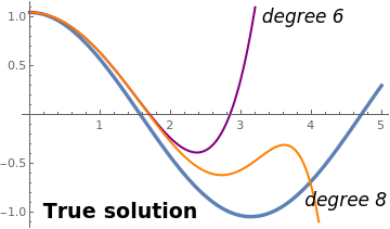
pendulum = Plot[Evaluate[theta[t] /. s], {t, 0, 5}, PlotStyle -> {Thickness[0.01]}]; t0 = Pi/3; c2 = -omega^2*Sin[t0]/2; A2 = c2*Cos[t0]; c4 = -omega^2 *A2/12; A4 = c4*Cos[t0] - (c2)^2 *Sin[t0]/2; c6 = -omega^2 *A4/30; A6 = Simplify[c6*Cos[t0] - c2*c4*Sin[t0]]; c8 = -omega^2*A6/8/7; p6[t_] = (t0 + c2*t^2 + c4*t^4 + c6*t^6) /. omega -> 1 p8[t_] = (t0 + c2*t^2 + c4*t^4 + c6*t^6 + c8*t^8) /. omega -> 1 pp6 = Plot[p6[t], {t, 0, 30}, PlotRange -> {{0, 5}, {-1.1, 1.1}}, PlotStyle -> {Purple, Thick}]; pp8 = Plot[p8[t], {t, 0, 30}, PlotRange -> {{0, 5}, {-1.1, 1.1}}, PlotStyle -> {Orange, Thick}]; txt = Graphics[{Black, Text[Style["True solution", Bold, 18], {1.3, -1}]}]; txt6 = Graphics[{Black, Text[Style["degree 6", Italic, 16], {3.9, 1}]}]; txt8 = Graphics[{Black, Text[Style["degree 8", Italic, 16], {4.5, -0.88}]}]; Show[pendulum, pp6, pp8, txt, txt6, txt8] |
|
| True solution and two Adomian polynomial approximations. | Mathematica code |
Here is Mathematica code from Duan & rach (2011) article:
Example: We consider a version of Troesch’s problem
- Duan, J.-S., Rach, R., New higher-order numerical one-step methods based on the Adomian and the modified decomposition methods, Applied Mathematics and Computation, 2011, Vol. 218, Issue 6, pp. 2810--2828. https://doi.org/10.1016/j.amc.2011.08.024
- Roberts, S.M., Shipman, J.S., On the closed form solution of Troesch’s problem, Journal of Computational Physics, 1976, Vol. 21,, Issue 3, pp. 291--304.
Return to Mathematica page
Return to the main page (APMA0330)
Return to the Part 1 (Plotting)
Return to the Part 2 (First Order ODEs)
Return to the Part 3 (Numerical Methods)
Return to the Part 4 (Second and Higher Order ODEs)
Return to the Part 5 (Series and Recurrences)
Return to the Part 6 (Laplace Transform)
Return to the Part 7 (Boundary Value Problems)