The method of Picard iterations was the first method that was used to
prove the existence of solutions to initial value problems for Ordinary
Differential Equations (ODEs). It is not practical because every
iteration repeats the same calculation, slowing down the overall
process. Every iteration brings more accuracy to the
approximation, unless a stabilized point has been reached (when a
given iteration is equal to the previous one). Practical applications
usually apply to polynomial slope functions. Otherwise, it becomes
impossible to integrate. Thus, Picard's iterations are used mostly for
theoretical applications, as proven existence of solutions to an initial value
problem.
In this section, we discuss so called Picard's iteration method that was
initially used to prove the existence of an initial value problem (see
section in this tutorial). Although this method is not
of practical interest and it is rarely used for actual determination of a
solution to the initial value problem, nevertheless, there are known some
improvements in this procedure that make it practical. Picard's iteration is
important for understanding the material because it leads to an equivalent
integral formulation useful in establishing many numerical methods. Also,
Picard's iteration helps in developing algorithmic thinking when the user
implements it in a computer.
Return to computing page for the first course APMA0330
Return to computing page for the second course APMA0340
Return to Mathematica tutorial for the first course APMA0330
Return to Mathematica tutorial for the second course APMA0340
Return to the main page for the course APMA0330
Return to the main page for the course APMA0340
The derivative operator \( \texttt{D} = {\text d}/{\text d}x
\) is an unbounded operator because it could transfer a bounded
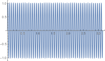
function into unbounded function. For example, the bounded and smooth function
sin(ωt) is mapped by the derivative operator into the unbounded
function ωcos(ωt), which may exceed any number upon
choosing an appropriate value of ω. This example shows that a fast
oscillating function may have a very large derivative, so its finite difference
approximation will be problematic. The same effect is observed when
the solution of a differential equation may be unbounded at some
point. Therefore, a practical approximation of such functions may not
be accurate unless we know that a solution is a smooth varying function. As an alternative, we try to reformulate
the initial value problem as an integral equation.
The inverse of the derivative operator \( \texttt{D} \) is not an operator in a general mathematical sense because it assigns to every function infinitely many outputs that are usually called an «antiderivative». In order to single out one output, we consider the differential operator on a special set of functions that have a prescribed value at one point x = x0, so f(x0) = y0. We change the notation \( \texttt{D} \) on such a set of functions (which is not a linear space) to L.
If we rewrite our initial value problem in the operator form \( L[y] = f , \) then apply its inverse L-1 to both sides, we reduce the given problem to the fixed point problem
\[
y = L^{-1} \left[ f(x,y) \right]
\]
for a bounded operatorL-1. If the given initial value problem is homogeneous, then Banach's or Brouwer's fixed point theorem assures us that for some bounded operators (such as L-1f for the Lipschitz slope function f) the iteration \( y_{n+1} = L^{-1} \left[ f(x,y_n ) \right] , \ y_0 = y(x_0 ) \) converges to a true solution. So Picard's iteration is actually an extension and implementation of this contraction theorem.
Banach’s
fixed point theorem formulates an easy-to-check assumption under which we have existence and uniqueness and comparability of a fixed point guaranteed. Moreover, it presents the order of the convergence of the approximating sequence and gives hints to stop the iteration in finitely many steps.
If we integrate (that is, apply the inverse
operator L-1 to the unbounded derivative operator restricted on the set of functions with a specified initial condition) both sides of the differential equation
\( y' = f(x,y) \) with respect to x from
x0 to x, we get
the following integral equation
The right-hand side of the (Volterra)
integral
equation above is actually the inverse operator
generated by the initial value problem. Therefore, both problems, the initial
value problem and its integral reformulation, are equivalent in the sense that
every solution of one of them is also a solution of its counterpart and vise
versa. Although this integral equation is
very hard (if not impossible) to solve, it has some advantages over the initial
value problem. The main feature of the integral equation is that it contains
integration---a bounded operator. This should be almost obvious for everyone
who took an introductory calculus course: integration (of a positive function)
is an area under the curve, which cannot be infinite for any smooth and
bounded function on a finite interval.
Now we deal with the fixed point problem that is more computationally
friendly because we can approximate an integral with any accuracy we want.
The Picard iterative process consists of constructing a sequence of
functions { ϕn } that will get
closer and closer to the desired solution. This is how the process works:
Then the limit function
\( \phi (x) = \lim_{n\to \infty} \phi_n (x) \)
gives the solution of the original initial value problem. However, practical implementation of Picard's iteration is possible only when the slope function is a polynomial. Otherwise, explicit integration is most likely impossible to achieve, even for a very sophisticated computer algebra system. We will show in the second part how to bypass this obstacle.
Theorem: Suppose that the slope
function f satisfies the existence and uniqueness theorem
(Picard--Lindelöf) in some rectangular domain \( \displaystyle R = [x_0 -a, x_0 +a]\times [y_0 -b , y_0 +b ] : \)
The slope function is bounded: \( M = \max_{(x,y) \in R} \, |f(x,y)| . \)
The slope function is Lipschitzcontinuous:
\( |f(x,y) - f(x,z) | \le L\,|y-z| . \) for all
(x,y) from R.
converges to the unique solution of the initial value problem
\( y' = f(x,y) , \ y(x_0 ) = y_0 , \) in the
interval \( x_0 - h \le x \le x_0 +h , \) where
\( \displaystyle h = \min \left\{ a, \frac{b}{M} \right\} . \)
⧫
If we chose the initial approximation as
\( \phi_0 (x_0 ) = y_0 , \) then at least the
initial condition \( y( x_0 ) = y_0 \) is
satisfied. The next approximation is obtained by substituting the initial
approximation into the right hand side of integral equation:
In this manner, we generate the sequence of functions
\( \displaystyle \left\{ \phi_n (x) \right\} = \left\{ \phi_0 , \phi_1 (x), \phi_2 (x) , \ldots \right\} . \)
Each member of this sequence satisfies the initial condition, but in general none satisfies the differential equation. If for some index m, we find that
\( \displaystyle \phi_{m+1} (x) = \phi_m (x) , \) then ϕm(x) is a fixed point of the integral equation
and it is a solution of the differential equation as well. Hence, the sequence is terminated at this point.
First, we verify that all members of the sequence exist. This follows from
the inequality:
The convergence of the sequence
\( \displaystyle \left\{ \phi_n (x) \right\} \)
is established by showing that the preseding infinite series converges.
To do this, we estimate the magnitude of the general term
\( \displaystyle \left\vert \phi_n (x) -
\phi_{n-1} (x) \right\vert \) .
where L is the Lipschitz constant for the function
f(x,y), that is,
\( \displaystyle \left\vert f(x, y_1 ) - f(x, y_2 )
\right\vert \le L \left\vert y_1 - y_2 \right\vert . \)
For the n-th term, we have
for any n. Hence, by the Weierstrass M-test, the series
\( \displaystyle
\phi (x) = \lim_{n\to \infty} \phi_n (x) = \phi_0 + \sum_{n\ge 1} \left[ \phi_n (x) - \phi_{n-1} (x) \right] \) converges absolutely and uniformly
on the interval \( \displaystyle \left\vert x - x_0 \right\vert \le h . \) Then it follows that the limit function
\( \displaystyle
\phi (x) = \lim_{n\to \infty} \phi_n (x) \) of the sequence
\( \displaystyle \left\{ \phi_n (x) \right\} \) is a
continuous function on the interval
\( \displaystyle \left\vert x - x_0 \right\vert \le h . \)
Next we prove that the limit function is a solution of the given initial value
problem. Allowing n to approach infinity on both sides of
Since the slope function satisfies the Lipschitz condition
\[
\left\vert f \left( t, \phi_n (t) \right) - f \left( t, \phi_{n-1} (t) \right)
\right\vert \le L \left\vert \phi_n (t) - \phi_{n-1} (t) \right\vert
\]
on the interval \( \displaystyle \left\vert t - x_0 \right\vert \le h , \)
it follows that the sequence
\( \displaystyle f \left( t, \phi_n (t) \right) \)
also converges uniformly to
\( \displaystyle f \left( t, \phi (t) \right) \)
on this interval. So we can interchange integration with the limit operation on the right-hand side to obtain
Thus, the limit function is a solution of the Volterra integral equation that is equivalent to the given initial value problem. Note that the limit function automatically satisfies the initial condition y(0) = y0.
Also, differentiating both sides of the latter with respect to x and noting that the right-hand side is a differentiable function of the upper limit, we find
\[
\phi' (x) = f(x, \phi (x)) .
\]
More details for the existence and uniqueness of the initial value problem
can be found in the following textbooks
Birkhoff, G. and Rota, G.-C., Ordinary Differential equations, 4rd Ed., John Wiley and Sons, New York, NY, 1989, Chapter 1, p. 23.
https://doi.org/10.1137/1005043
Wouk, A., On the Cauchy-Picard Method, The American Mathematical Monthly, Vol. 70, No. 2. (Feb., 1963), pp. 158-162.
▣
Although this approach is most often connected with
the names of Charles Emile Picard, Giuseppe Peano, Ernst Lindelöf, Rudolph Lipschitz, and Augustin Cauchy, it
was first published by the French mathematician Joseph Liouville in 1838 for solving second order homogeneous linear equations. About fifty years later, Picard developed a much more generalized form, which placed the concept on a more rigorous mathematical foundation, and used this approach to solve boundary value problems described by second order ordinary differential equations.
Note that Picard's iteration procedure, if it could be performed,
provides an explicit solution to the initial value problem. This
method is not for practical applications mostly for two reasons:
finding the next iterate may be impossible, and, when it works, Picard's iteration contains repetitions. Therefore, it could be used sometimes for approximations only. Moreover, the interval of existence (-h, h) for the considered initial value problem is in most cases far away from the validity interval. Some improvements in this direction are known (for instance, S.M. Lozinsky theorem), but we are far away from a complete determination of the validity interval based on Picard's iteration procedure. Also, there are a number of counterexamples in
which the Picard iteration is guaranteed not to converge, even if the starting function is arbitrarily close to the real solution.
Here are some versions of Picard's iteration procedure for Mathematica:
For[{n = 1, y[0][x_] = 1}, n < 4, n++, y[n][x_] = 1 + Integrate[y[n - 1][t]^2 + t^2, {t, 0, x}]; (* x^2 + y^2 is taken for example *)
Print[{n, y[n][t]}]]
The iteration step is called iterate, and it keeps track of the iteration order n so that it can assign a separate integration variable name at each step. As additional tricks to speed things up, I avoid the automatic simplifications for definite integrals by doing the integral as an indefinite one first, then using Subtract to apply the integration limits.
Instead of a generic simplification, I add Expand to the result in order to help the subsequent integration step recognize how to split up the integral over the current result. The last argument in iterate is the name that I intend to use as the base variable name for the integration, but it will get a subscript n attached to it.
Then iterate is called by picardSeries, using increasing subscripts starting with the outermost integration. This is implemented using Fold with a Reverse range of indices. The first input is the initial condition, followed by the function defining the flow (specifically, defined below as flow[t_, f_]). After the order n, I also specify the name of the independent variable var as the last argument.
Here is the example applied to the IVP: \( y' = y^2 + x^2 , \ y(0) =1 . \)
Since the initial ieteration is identically zero, all other terms become zero as well. So Picard's iteration provides the trivial solution---identically zer. On the other hand, the function
\[
y = \phi (x) = \left( \frac{2}{3}\, x \right)^{2/3}
\]
is another solution, which is a singular solution.
We make a conclusion that continuity of a slope function is unsufficient for the conclusion that there exists a unique solution---it is sufficient for existence of the solution.
Let us consider another slope function
\[
f(x,y) = \begin{cases}
0, & \ x=0, \quad -\infty < y < \infty \\
2x, & \ 0 < y \le 1, \quad -\infty < y < 0, \\
2x - \frac{4y}{x} , & \ 0 < x \le 1, \quad 0 \le y \le x^2 \\
-2x & \ 0 < x \le 1, \quad x^2 < y < +\infty ,
\end{cases}
\]
for 0 ≤ x ≤ 1. −∞ < y < ∞.
It is clear that the slope function is continuous and bounded by the constant 2. Using the initial approximation ϕ0 = 0, we obtain two sequences defined on the interval [0, 1]:
Therefore, the sequence of Picard's iterations has two cluster values for each x ≠ 0, and it does not converge because neither of the functions ϕ2k and ϕ2k-1 is a solution of the given differential equation.
■
Example:
Consider the initial
value problem for the linear equation
and so on. So we see that first terms stabilize with each iteration, and we hope to achieve the explicit solution (expansion). We check with Mathematica:
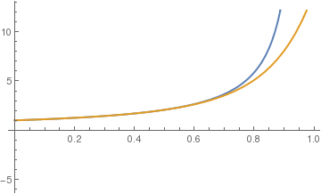
Picard 4th iteration and explicit solution
Plotted figure shows a good approximation on the interval about [0,0.7]. Picard's theorem guarantees the existence of solution on the interval \( [0, 1/\sqrt{2}) \approx (0,0.7) , \) which is far away from the root 0.969811, where the denominator is zero.
■
Example:
Consider the initial
value problem for the
Riccatiequation
There are some discrepancies in coefficients; however, Picard's theorem guarantees that they will eventually go away, and the series will be stabilized.
■
Example:
Practically, the Picard iteration scheme can be implemented only when slope function is a polynomial because this is the only functions that we integrate explicitely for its compositions. The following example shows that an equation containing a radical prevents of explicit integrations required by Picard's iteration.
Consider the initial
value problem for the autonomous equation
Bai, X., Junkins, J.: Modified Chebyshev--Picard iteration methods for solution of initial value problems, The Journal of the Astronautical Sciences volume 59, 327–351 (2011)
Bai, X., Junkins, J.: Modified Chebyshev--Picard iteration methods for solution of boundary value problems. The Journal of the Astronautical Sciences, 58, 615–642 (2011)
Fabrey, J., Picard's theorem,
The American Mathematical Monthly, 1972,Vol. 79, No. 9, pp. 1020--1023
Lozinski, S.M., On a class of linear operators, Dokladu Akademii Nauk SSSR, 1948, Vol. 61, pp. 193-196. (Russian)
Robin, W.A., Solving differential equations using modified Picard iteration, International Journal of Mathematical Education, 2010, Vol. 41, No. 5, pp. 649--665; doi: 10.1080/00207391003675182
Tisdell, Christopher C.,
Improved pedagogy for linear differential equations by reconsidering how we measure the size of solutions,
International Journal of Mathematical Education, 2017, Vol. 48, Issue 7, pp. 1087--1095;
https://doi.org/10.1080/0020739X.2017.1298856
Tisdell, Christopher C., On Picard's iteration method to solve differential equations and a pedagogical space for otherness, International Journal of Mathematical Education, 2018, https://doi.org/10.1080/0020739X.2018.1507051
Youssef, I.K., "Picard iteration algorithm combined with Gauss--Seidel technique for initial value problems," Applied Mathematics and Computation, 2007, 190, 345--355.
Return to Mathematica page
Return to the main page (APMA0330)
Return to the Part 1 (Plotting)
Return to the Part 2 (First Order ODEs)
Return to the Part 3 (Numerical Methods)
Return to the Part 4 (Second and Higher Order ODEs)
Return to the Part 5 (Series and Recurrences)
Return to the Part 6 (Laplace Transform)
Return to the Part 7 (Boundary Value Problems)