Preface

---

This section discusses some practical algorithms for finding a point p in the general equation of the form p = g(p), for some continuous function g(x). Existence of solution to the equation above is known as the fixed point theorem, and it has numerous generalizations. This theorem has many applications in mathematics and numerical analysis. For instance, Picard's iteration and Adomian decomposition method are based on fixed point theorem.

Fixed Point Iteration

---

Iteration is a fundamental principle in computer science. As the name suggests, it is a process that is repeated until an answer is achieved or stopped. In this section, we study the process of iteration using repeated substitution.

More specifically, given a function g defined on the real numbers with real values and given a point x₀ in the domain of g, the fixed point (also called Picard's) iteration is

which gives rise to the sequence \( \left\{ x_i \right\}_{i\ge 0} . \) If this sequence converges to a point x, then one can prove that the obtained x is a fixed point of g, namely,

One of the most important features of iterative methods is their convergence rate defined by the order of convergence. Let { x_n } be a sequence converging to α and let ε_n = x_n - α.

When one wants to apply a function until the result stops changing, Mathematica provides dedicated commands FixedPoint and FixedPointList to achieve that. We present an alternative approaches. One can also use NSolve command, as the following example shows. Example 1: transcendent equation Example 2: polynomial equation Example 3: convergent iteration Example 4: rational function Stefan Banach (was born in 1892 in Kraków, Austria-Hungary and died 31 August 1945 in Lvov, Ukrainian SSR, Soviet Union) was a Polish mathematician who is generally considered one of the world's most important and influential 20th-century mathematicians. He was one of the founders of modern functional analysis, and an original member of the Lwów School of Mathematics. His major work was the 1932 book, Théorie des opérations linéaires (Theory of Linear Operations), the first monograph on the general theory of functional analysis.
Rudolf Otto Sigismund Lipschitz (1832--1903) was a German mathematician who made contributions to mathematical analysis (where he gave his name to the Lipschitz continuity condition) and differential geometry, as well as number theory, algebras with involution and classical mechanics. In practice, it is often difficult to check the condition \( g([a,b]) \subset [a,b] \) given in the previous theorem. We now present a variant of it.

Remark: If g is invertible then P is a fixed point of g if and only if P is a fixed point of g^-1.

Remark: The above theorems provide only sufficient conditions. It is possible for a function to violate one or more of the hypotheses, yet still have a (possibly unique) fixed point. ■

The Banach theorem allows one to find the necessary number of iterations for a given error "epsilon." It can be calculated by the following formula (a-priori error estimate)

and a-posteriori error estimate (where p is a fixed point):

 

Example 5: rational function Example 6: trig function Example 7: another trig function

 

Sometimes we can accelerate or improve the convergence of an algorithm with very little additional effort, simply by using the output of the algorithm to estimate some of the uncomputable quantities. One such acceleration was proposed by A. Aiken. Alexander Craig "Alec" Aitken was born in 1895 in Dunedin, Otago, New Zealand and died in 1967 in Edinburgh, England, where he spent the rest of his life since 1925. Aitken had an incredible memory (he knew π to 2000 places) and could instantly multiply, divide and take roots of large numbers. He played the violin and composed music to a very high standard.

Suppose that we have an iterative process that generates a sequence of numbers \( \{ x_n \}_{n\ge 0} \) that converges to α. We generate a new sequence \( \{ q_n \}_{n\ge 0} \) according to

where \( \Delta x_n = x_{n+1} - x_n \) is the forward difference. Corespondingly, the backward difference is

This algorithm was proposed by one of New Zealand's greatest mathematicians Alexander Craig "Alec" Aitken (1895--1967). When it is applied to determine a fixed point in the equation \( x=g(x) , \) it consists in the following stages:

• select x₀;
• calculate
  \[ x_1 = g(x_0 ) , \qquad x_2 = g(x_1 ) ; \]
• calculate
  \[ x_3 = x_2 + \frac{\gamma_2}{1- \gamma_2} \left( x_2 - x_1 \right) , \qquad \mbox{where} \quad \gamma_2 = \frac{x_2 - x_1}{x_1 - x_0} ; \]
• calculate
  \[ x_4 = g(x_3 ) , \qquad x_5 = g(x_4 ) ; \]
• calculate x₆ as the extrapolate of \( \left\{ x_3 , x_4 , x_5 \right\} . \) Continue this procedure, ad infinatum. ■ 

We assume that g is continuously differentiable, so according to Mean Value Theorem there exists ξ_n-1 between α (which is the root of \( \alpha = g(\alpha ) \) ) and x_n-1 such that

Now consider so that solving for α implies

Since we are assuming that \( x_n \,\to\, \alpha , \) we also know that \( g' (\xi_n ) \, \to \,g' (\alpha ) ; \) thus, we can denote \( \gamma_n \approx g' (\xi_{n-1} ) \approx g' (\alpha ) . \) Using this notation, we get

which we use to define a new sequence of approximations: Example 8: exponential function Now we present version 1 of Aitken extrapolation that does not take as much advantage of acceleration as is possible. Aitken Extrapolation, Version 1
x1 = g(x0)
x2 = g(x1)
for k=1 to n do
if (dabs[x1 - x0) > 1.d-20) then
gamma = (x2 - x1)/(x1 - x0)
else
gamma = 0.0d0
endif
q = x2 + gamma*(x2 - x1)/(1 - gamma)
if(abs(q - x2) < error) then
alpha = q
stop
endif
x = g(x2)
x0 = x1
x1 = x2
x2 = x
enddo
Since division by zero---or a very small number---is possible in the algorithm's computation of γ, we put in a conditional test: Only if the denominator is greater than 10^-20 do we carry through the division. Example 9: to be done

 

Johan Frederik Steffensen (1873--1961) was a Danish mathematician, statistician, and actuary who did research in the fields of calculus of finite differences and interpolation. He was a professor of actuarial science at the University of Copenhagen from 1923 to 1943. Steffensen's inequality and Steffensen's iterative numerical method are named after him.

When Aitken's Δ² process is combined with the fixed point iteration, the result is called Steffensen's acceleration. Starting with p₀, two steps of iteration procedure should be performed

Then we compute At this point, we ``restart'' the fixed point iteration with \( p_0 = q_0 , \) e.g., and compute If at some point \( \Delta^2 p_n =0 \) (which appears in the denominator), then we stop and select the current value of p_n+2 as our approximate answer.

Steffensen's acceleration is used to quickly find a solution of the fixed-point equation x = g(x) given an initial approximation p₀. It is assumed that both g(x) and its derivative are continuous, \( | g' (x) | < 1, \) and that ordinary fixed-point iteration converges slowly (linearly) to p.

Example 10: Transcendent function (divergence) Example 11: Transcendent function (convergence)

 

To solve the fixed point problem \( g(x) =x , \) the following algorithm, presented by J.H. Wegstein in 1958, can be used Till some extend, Wegstein's method is a version of predictor-corrector method because it can be broken into two stages: for \( n=0,1,2,\ldots . \) Wegstein (1958) found that the iteration converge differently depending on the value of q.

q < 0	Convergence is monotone
0 < q < 0.5	Convergence is oscillatory
0.5 < q < 1	Convergence
q > 1	Divergence

Wegstein's method depends on two first guesses x⁰ and x¹ and poor start may cause the process to fail, converge to another root, or, at best, add unnecessary number of iterations. Example 12: to be done

 

Mark Krasnosel'skii		William Robert Mann

There are several iteration techniques for approximating fixed points equations of various classes. The Picard’s iteration technique, the Mann iteration technique and the Krasnosel’skii iteration technique are the most used of all those methods. Mark Alexandrovich Krasnosel'skii (1920--1997) was a Soviet, Russian mathematician renowned for his work on nonlinear functional analysis and its applications. William Robert Mann (1920--2006) was a mathematician from Chapel Hill, North Carolina, USA. The K--M algorithm is used to a fixed point equation

where T is a self-mapping of a closed subset. The K--M algorithm generates a sequence { x_m } according to the recursive formula where α_n is a sequence in the interval (0,1) and the initial guess x₀ is chosen arbitrary. Obviously, for the special case α_n =1, the Krasnosel’skii--Mann iterative scheme results in Picard's method. Example 13: to be done

 

The Adomian decomposition method (ADM) is a method for solving nonlinear equations. The crucial step of this method includes the decomposition of the nonlinear term into so called Adomian's polynomials.

Consider the nonlinear equation f(x) = 0, which can be transformed into

where g(x) is a nonlinear function, which is assumed to have as many derivatives as needed. Let x = c be an estimated root of the above equation x = g(x). By making a shift u = x - c, we transfer the given fixed problem to the following one: The above equation is more friendly for the Adomian decomposition method (ADM for short) because u has small value, so u₀ = 0 will be its initial approximation. Then we represent u as the series that is assumed to converge: Hence, the initial approximation is zero: u₀ = 0, which corresponds to x₀ = c. The nonlinear term g(u+c) can be also decomposed into the Adomian polynomials, which leads to the equation where the A_i's are the Adomian polynomials: First few of these polynomials can be generated as follows: The following Mathematica code was prepared by Jun-Sheng Duan: Now we calculate each term in the sum for x recursively:

Since u_n+1 = A_n, we represent the required solution of the fixed point problem x = g(x) as

Five term approximation becomes Depending on the initial approximation c, we can calculate its 5-term Adomian approximation using the following Mathematica code

The ADM does not assure the existence and uniqueness of solutions, but it can be safely applied in cases when a fixed point theorem holds. This will be demonstrated in the following examples.

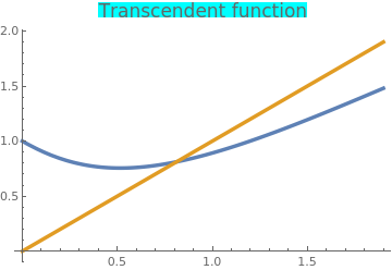
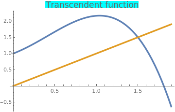
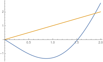
Example 14: Adomian's polynomails for the resiprocal Example 15: Adomian method solves the quadratic equation Example 16: Failing find a root of a transcendent equation Example 17: Root of a transcendent equation

 

References on papers related to fixed point iteration

 

 

Return to Mathematica page
Return to the main page (APMA0330)
Return to the Part 1 (Plotting)
Return to the Part 2 (First Order ODEs)
Return to the Part 3 (Numerical Methods)
Return to the Part 4 (Second and Higher Order ODEs)
Return to the Part 5 (Series and Recurrences)
Return to the Part 6 (Laplace Transform)
Return to the Part 7 (Boundary Value Problems)