Preface


This section discusses a completely different strategy to solve an initial value problem for a single first-order differential equation \( y' = f(x,y) , \quad y(x_0 )= y_0 . \) In order to calculate an approximate value of the solution φ(tn+1) at the next mesh point t = tn+1, the values of the calculated solution at some previous mesh points are used. The numerical methods that use information at more than the last mesh point are referred to as multistep methods. This section presents two types of multistep methods: Adams methods and backward differentiation methods. Different levels of accuracy can be achieved with each type of methods.

Return to computing page for the first course APMA0330
Return to computing page for the second course APMA0340
Return to Mathematica tutorial for the second course APMA0340
Return to the main page for the course APMA0330
Return to the main page for the course APMA0340
Return to Part III of the course APMA0330

Variational Iteration Method


Ji-Huan He

Recently, there has been great development of new powerful methods capable of handling linear and nonlinear equations. Among them, there are known the Adomian decomposition method (ADM), the variational iteration method, and the homotopy perturbation method. The variational iteration method (VIM, for short) was developed by Ji-Huan He in 1999--2007. This method is preferable over numerical methods as it is free from rounding off errors as it does not involve discretization and does not require large computer power or memory. The VIM gives rapidly convergent successive approximations of the exact solution if such a solution exists; otherwise, a few approximations can be used for numerical purposes. Unlike the ADM, where computational algorithms are normally used to deal with nonlinear terms, the VIM does not require the utilization of restrictive assumptions because it approaches linear and nonlinear problems directly in a like manner. Many researches in variety of scientific fields applied this method and showed the VIM has many merits and to be reliable for a variety of scientific application. In particular, Abassy et al., proposed the modified variational iteration method (MVIM) to avoid repeated computation of redundant terms.

To illustrate the basic concept of the He’s VIM, consider the following general nonlinear equation:

\[ L\left[ y(x) \right] = N\left[ y(x) \right] + g(x) , \]
where \( L = \texttt{D} = {\text d}/{\text d}x \) is the linear differential operator (which in general can include other terms), N is the nonlinear operator, and g is the input (known) function. He has modified the general Lagrange multiplier method to an iteration method called as correction functional. The basic character of the method is to construct a correction functional for the aforementioned equation, which reads as
\[ y_{n+1} (x) = y_n (x) + \int_0^x \lambda (s) \left\{ L\left[ y_n (s) \right] - N\left[ \tilde{y}_n (s) \right] - g(s) \right\} {\text d}s , \]
where λ is a Lagrange multiplier. The subscript n denotes the n-th approximation, and \( \tilde{y}_n \) is a restricted variation., i.e., \( \delta\tilde{y}_n = 0 . \) We start our exposition with the linear case:
\[ y' (x) + p(x)\, y = g(x) , \qquad y(0) = \alpha . \]
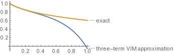
According to the VIM, the basic character of the method is to construct a correction functional for the equation, which reads
\[ y_{n+1} (x) = y_n (x) + \int_0^x \lambda (s) \left\{ y'_n (s) + p(s)\, \tilde{y}_n (s) - g(s)\right\} {\text d}s , \qquad n=0,1,2,\ldots . \]
Here λ(s,x) is so called a general Lagrange multiplier, which can be identified optimally via variational theory, and \( \tilde{y}_n \) denotes a restricted variation, that is, \( \delta\tilde{y}_n =0. \) Having λ obtained, an iteration formula should be used for the determination of the successive approximations yn+1(t) of the solution y(t). The initial approximation y0(t) can be arbitrary function; however, it is usually selected based on the initial conditions. Consequently, the solution is given by
\[ y(x) = \lim_{n\to\infty}\,y_n (x) . \]

The main problem for obtaining highly accurate solutions with the VIM is the determination of the Lagrange multiplier, and there are known many forms of them. This parameter plays the important role in the speed of convergence of the VIM solution. Finding the Lagrange multiplier could be achieved by making the correction functional stationary. Taking variation with respect to the variable yn, noticing δyn(0)=0, we get

\begin{eqnarray*} \delta y_{n+1} (x) &=& \delta y_n (x) + \delta \int_0^x \lambda \left\{ y'_n (s) + \tilde{y}_n (s) - g(s) \right\} {\text d}s \\ &=& \delta u_n (x) + \left. \lambda\,\delta y_n \right\vert_{s=x} + \int_0^x \left[ -\lambda ' \delta y_n \right] {\text d}s =0 , \end{eqnarray*}
for all variations δyn. This yields the following equation
\[ \left. \lambda ' \right\vert_{s=x} =0 \qquad\mbox{and} \qquad \left. 1+ \lambda \right\vert_{s=x} =0 . \]
Solving the above equations, we obtain λ = -1, and the correction functional gives the iteration formula
\[ y_{n+1} (x) = y_n (x) - \int_0^x \left\{ y'_n (s) + p(s)\,y_n (s) - g(s) \right\} {\text d}s , \qquad n=0,1,2,\ldots . \]
Originally, Ji-Huan He did not consider the linear part as a restricted variation and applied it only to nonlinear terms. Furthermore, the lesser the application of restricted variations the faster the approximations converging to its exact solution. In this case, he obtained (using integration by parts) the following equations for λ determination:
\[ \begin{split} -\lambda ' (s) + p(s)\,\lambda (s) &=0 , \\ 1 + \left. \lambda (s) \right\vert_{s=t} &= 0. \end{split} \]
Solving the above equations with Mathematica,
DSolve[{lambda'[s] == p[s]*lambda[s], lambda[x] == -1}, lambda[s], s]
we obtain another formula for the Lagrange multiplier
\[ \lambda (s,x) = - \exp \left\{ \int_x^s p(\tau )\,{\text d} \tau \right\} . \]
In both approaches, there are repeated calculations in each step (similar to Picard's method); to cancel some of the repeated calculations, the iteration formula can be handled as follows.
\[ y_{n+1} = y_n - \int_0^x y'_n (s)\, {\text d}s - \int_0^x \left\{ p(s)\,y_n (s) - g(s) \right\} {\text d}s , \qquad n=0,1,2,\ldots . \]
Hence,
\[ y_{n+1} = y_n (0) - \int_0^x \left\{ p(s)\,y_n (s) - g(s) \right\} {\text d}s , \qquad n=0,1,2,\ldots . \]
We can set \( y_n (0) = y_0 = \alpha , \) so
\[ y_{n+1} = y_0 - \int_0^x \left\{ p(s)\,y_n (s) - g(s) \right\} {\text d}s , \qquad n=0,1,2,\ldots . \]
To eliminate all repeated computations, let us rewrite the latter in the following iteration formula:
\[ y_{n+1} = y_0 - \int_0^x \left\{ p(s)\left( y_n (s) - y_{n-1} (s) \right) \right\} {\text d}s - \int_0^x \left\{ p(s)\,y_{n-1} (s) -g(s) \right\} {\text d}s , \qquad n=0,1,2,\ldots . \]
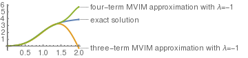
Using the identity \( y_{n} = y_0 - \int_0^x \left\{ p(s)\,y_{n-1} (s) - g(s) \right\} {\text d}s , \) we obtain so called the modified variational iteration formula:
\[ y_{n+1} = y_n - \int_0^x \left\{ p(s)\left( y_n (s) - y_{n-1} (s) \right) \right\} {\text d}s , \qquad n=0,1,2,\ldots . \]
We proceed further iterations based on \( y_{0} = y(0) = \alpha , \ y_{-1} =0 . \) Now it is right time to show how it works in a series on examples.

Example: Consider the IVP for the linear differential equation

\[ y' -y = \sin x , \qquad y(0) =1 . \]
Mathematica easily find its solution:
DSolve[{y'[x] == y[x] + Sin[x], y[0] == 1}, y[x], x]// Flatten
\[ y(x) = \frac{1}{2} \left( 3\,e^x - \cos x - \sin x \right) = 1 + x + x^2 + \frac{x^3}{3} + \frac{x^4}{24} + \frac{x^5}{5!} + \frac{x^6}{360} + \cdots . \]
For solving this initial value problem by MVIM, we set \( y_{-1} =0, \ y_0 =1 . \) Then we use the following iterative formula
\[ y_{n+1} = y_n + \int_0^x \left\{ y_n (s) - y_{n-1} (s) \right\} {\text d}s , \qquad n=0,1,2,\ldots . \]
The first term needs a special attention.
\[ y_{1} (x) = y_0 + \int_0^x \left\{ y_0 (s) - y_{-1} (s) + \sin s \right\} {\text d}s = 2 +x - \cos x . \]
Other terms are calculated according to the above formula.
\begin{eqnarray*} y_{2} (x) &=& y_1 + \int_0^x \left[ y_1 (s) - y_0 (s) \right] {\text d}s = \frac{1}{2} \left( 2+x \right)^2 - \cos x - \sin x , \\ y_{3} (x) &=& y_2 + \int_0^x \left[ y_2 (s) - y_1 (s) \right] {\text d}s = \left( 1+x \right)^2 + \frac{x^3}{6} - \sin x = 1 + x + x^2 + \frac{x^3}{3} + \frac{x^4}{24} - \frac{x^5}{5!} + \cdots , \\ y_{4} (x) &=& y_3 + \int_0^x \left[ y_3 (s) - y_2 (s) \right] {\text d}s = 1 + x + x^2 + \frac{x^3}{3} + \frac{x^4}{24} , \end{eqnarray*}
and so on.
y1[x_] = 1 + Integrate[1 + Sin[s], {s, 0, x}];
y2[x_] = y1[x] + Integrate[y1[s] - 1, {s, 0, x}];
y3[x_] = Simplify[y2[x] + Integrate[y2[s] - y1[s], {s, 0, x}]];
y4[x_] = Simplify[y3[x] + Integrate[y3[s] - y2[s], {s, 0, x}]];
We plot last two approximations along with the true solution.
exact[x_] = (3*Exp[x]-Cos[x]-Sin[x])/2 ;
Plot[{Callout[y4[x], "four-term VIM approximation"], Callout[y3[x], "three-term VIM approximation"], Callout[exact[x], "exact"]}, {x, 0, 3.5}, PlotStyle->Thick]
True solution and MVIM approximations with N = 3 and 4 terms.
   ■

Example: Consider the IVP for the generalized logistic equation

\[ \dot{u} = u \left( 2-u \right) \left( 4-u \right) , \qquad u(0) =1. \]
Here dot represents differentiation with respect to time variable. First, find its solution:
exact[t_] = u[t]/.DSolve[{u'[t] == u[t]*(2 - u[t])*(4 - u[t]), u[0] == 1}, u[t], t]
\[ u(t) = 2 \,\frac{1 + 3\, e^{8t} - \sqrt{1 + 3\, e^{8t}}}{1 + 3\, e^{8t}} = 1 + 3t - \frac{3}{2}\, t^2 - \frac{17}{2}\, t^3 + \frac{125}{8}\, t^4 + \frac{721}{40}\, t^5 - \frac{23401}{240}\, t^6 + \cdots . \]
In the hybrid model, u(t) is the portion of population of a certain characteristic, and t is the time measured in generations.

Since the Lagrange multiplier is λ = -1, we have the following recurrence:

\[ u_{n+1} = u_n - \int_0^x \left\{ u'_n (s) - u_n (s) \left( 2-u_n (s) \right) \left( 4-u_n (s) \right) \right\} {\text d}s , \qquad n=0,1,2,\ldots . \]
Since the given differential equation is homogeneous, we don't need to distinguish u1 from other terms. Settingu0 to be the initial value, we have
\begin{eqnarray*} u_{0} (t) &=& 1, \\ u_1 (t) &=& u_0 + \int_0^t \left\{ u_0 (s) \left( 2-u_0 (s) \right) \left( 4-u_0 (s) \right) \right\} {\text d}s = 1+ 3t , \\ u_2 (t) &=& u_1 - \int_0^t \left\{ u'_1 (s) - u_1 (s) \left( 2-u_1 (s) \right) \left( 4-u_1 (s) \right) \right\} {\text d}s = 1+ 3t - \frac{3}{2}\, t^2 - 9\,t^3 + \frac{27}{4} \, t^4 , , \\ u_3 (t) &=& u_2 - \int_0^t \left\{ u'_2 (s) - u_2 (s) \left( 2-u_2 (s) \right) \left( 4-u_2 (s) \right) \right\} {\text d}s = 1+ 3t - \frac{3}{2}\, t^2 - 9\,t^3 + \frac{27}{4} \, t^4 , , \\ u_4 (t) &=& u_3 - \int_0^t \left\{ u'_3 (s) - u_3 (s) \left( 2-u_3 (s) \right) \left( 4-u_3 (s) \right) \right\} {\text d}s = 1+ 3t - \frac{3}{2}\, t^2 - 9\,t^3 + \frac{27}{4} \, t^4 , , \end{eqnarray*}
and so on.
u1[t_] = 1 + 3*t;
u2[t_] = u1[t] - Integrate[D[u1[s], s] - u1[s]*(2 - u1[s])*(4 - u1[s]), {s, 0, t}];
u3[t_] = u2[t] - Integrate[D[u2[s], s] - u2[s]*(2 - u2[s])*(4 - u2[s]), {s, 0, t}];
u4[t_] = u3[t] - Integrate[D[u3[s], s] - u3[s]*(2 - u3[s])*(4 - u3[s]), {s, 0, t}]
We plot last two approximations along with the true solution.
Plot[{Callout[u4[t], "four-term VIM approximation"], Callout[u3[t], "three-term VIM approximation"], Callout[exact[t], "exact solution"]}, {t, 0, 1.4}, PlotStyle->Thick]
True solution and MVIM approximations with N = 3 and 4 terms.
   ■

Example: Consider the IVP for the following Riccati equation

\[ y' = 3\,y - y^2 + 2\,x, \qquad y(0) =0. \]
First, we write the variational iteration sequence:
\[ y_{n+1} (x) = y_n (x) + \int_0^x \lambda (x,s) \left\{ y'_n (s) - 3\,y_n (s) + \tilde{y}_n^2 - 2\,s \right\} {\text d}s , \qquad n=0,1,2,\ldots . \]
Taking variation, we obtain
\begin{eqnarray*} \delta y_{n+1} (x) &=& \delta y_n (x) + \delta \int_0^x \lambda \left\{ y'_n (s) - 3\,y_n (s) + \tilde{y}_n^2 - 2\,s \right\} {\text d}s \\ &=& \delta y_n (x) + \delta \int_0^x \lambda \left\{ y'_n (s) - 3\,y_n (s) \right\} {\text d}s \\ &=& \delta y_n (x) + \left. \lambda\,\delta y_n (s) \right\vert_{s=0}^{s=t} - \int_0^t \left[ \lambda ' + 3\,\lambda \right] \delta y_n (s) \, {\text d}s . \end{eqnarray*}
This gives us the equations for determination of the Lagrange multiplier:
\[ \begin{split} \lambda ' (s) + 3\,\lambda (s) &=0 , \\ 1 + \left. \lambda (s) \right\vert_{s=t} &= 0. \end{split} \]
So the multiplier can be identified as
\[ \lambda (x,s) = - e^{3(x-s)} . \]
Then the iteration formula becomes
\[ y_{n+1} = y_n - \int_0^x e^{3(x-s)} \left\{ y'_n (s) - 3\,y_n (s) + y_n^2 - 2\,s \right\} {\text d}s , \qquad n=0,1,2,\ldots . \]
Using previously defined subroutine seriesDSolve, we find series solution of the given problem:
seriesDSolve[ y'[x] == 2*x + 3*y[x] - (y[x])^2, y, {x, 0, 10}, {y[0] -> 0}]
\[ y = x^2 + x^3 + \frac{3}{4}\,x^4 + \frac{x^5}{4} - \frac{5}{24}\, x^6 - \frac{25}{56}\,x^7 - \frac{187}{448}\, x^8 - \frac{2551}{12096}\, x^9 + \frac{1217}{40320}\, x^{10} + \cdots . \]
We start with an initial approximation y0 = x². This yields
\begin{eqnarray*} y_1 (x) &=& x^2 - \int_0^x e^{3(x-s)} \left\{ 2s - 3\,s^2 + s^4 - 2\,s \right\} {\text d}s = x^2 + \frac{1}{81} \left( 27\,x^4 -45\,x^2 -30\,x -10 \right) + \frac{10}{81}\, e^{3x} , \\ y_2 (x) &=& y_1 - \int_0^x e^{3(x-s)} \left\{ y'_1 -3\,y_1 + y_1^2 -2\,s \right\} {\text d}s \approx x^2 - \frac{x^3}{3} - \frac{x^4}{4} - \frac{3}{20}\, x^5 - \frac{3}{40}\, x^6 + \frac{253}{840}\, x^7 + \cdots . \end{eqnarray*}
So we see that calculations become messy very shortly. We ask Mathematica for help.
y1[t_] = t^2 - Integrate[(s^4 - 3*s^2)*Exp[3*t - 3*s], {s, 0, t}];
y2[t_] = y1[t] - Integrate[(D[y1[s], s] - 3*y1[s] + (y1[s])^2 - 2*s)* Exp[3*t - 3*s], {s, 0, t}];
y3[t_] = y2[t] - Integrate[(D[y2[s], s] - 3*y2[s] + (y2[s])^2 - 2*s)* Exp[3*t - 3*s], {s, 0, t}];
Expand[y3[t]]
Series[%, {t, 0, 10}]
\[ y_3 (x) \approx x^2 + x^3 + \frac{3}{4}\,x^4 + \frac{x^5}{4} - \frac{5}{24}\, t^6 - \frac{25}{56}\, x^7 - \frac{187}{448}\, x^8 + \frac{2551}{12096} \, x^9 + \frac{1217}{40320}\, x^{10} + \cdots , \]
which gives the correct answer up to the power 10 (at least). Then we plot the third approximation y3 and the true solution.
sol = (y[x] /.
DSolve[{y'[x] == 2*x + 3*y[x] - (y[x])^2, y[0] == 0}, y[x], x])[[1]];
Plot[{Callout[sol, "exact"], Callout[y3[x], "three-term VIM approximation"]}, {x,0,1.4}, PlotStyle->Thick]
True solution and third VIM approximation.

We demonstrate a modified variational iteration method and choose the Lagrange multiplier as λ = -1. This leads in our case to the recurrence:

\[ y_{n+1} (t) = y_n (t) + 3 \int_0^t \left( y_n (s) - y_{n-1} (s) \right) {\text d}s - \int_0^t \left( y_n^2 (s) - y_{n-1}^2 (s) \right) {\text d}s , \qquad n=1,2,\ldots ; \]
where \( y_{-1} = 0, \ y_0 = 0 \) (from the initial condition). The first term should include the input function
\[ y_{1} (t) = y_0 + \int_0^t \left[ y'_0 (s) - 3 \, y_0 + y_0^2 - 2\,s \right] {\text d}s = t^2 . \]
Therefore, we can obtain the following successive approximations:
\begin{eqnarray*} y_2 (t) &=& t^2 + 3\, \int_0^t \left[ y_1 (s) - y_{0} \right] {\text d}s - \int_0^t \left[ y_1^2 - y_{0}^2 \right] {\text d}s = t^2 + t^3 - \frac{t^5}{5} , \\ y_3 (t) &=& y_2 (t) + 3\, \int_0^t \left[ y_2 (s) - y_{1} (s) \right] {\text d}s - \int_0^t \left[ y_2^2 (s) - y_{1}^2 (s) \right] {\text d}s = t^2 + t^3 + \frac{3}{4}\,t^4 - \frac{t^5}{5} - \frac{13}{30}\, t^6 - \frac{t^7}{7} + \frac{t^8}{20} + \frac{2}{45}\,t^9 - \frac{t^{11}}{275} , \\ y_4 (t) &=& y_3 (t) + 3\, \int_0^t \left[ y_3 (s) - y_{2} (s) \right] {\text d}s - \int_0^t \left[ y_3^2 (s) - y_{2}^2 (s) \right] {\text d}s = t^2 + t^3 + \frac{3}{4}\,t^4 - \frac{t^5}{5} - \frac{13}{30}\, t^6 - \frac{5}{14}\, t^7 - \frac{11\,t^8}{80} + \frac{169}{2160}\,t^9 + \frac{61}{420} \, t^{10} + \cdots . \end{eqnarray*}
y2[t_] = t^2 + t^3 - t^5 /5
y3[t_] = y2[t] + Integrate[3*y2[s] - 3*s^2 - (y2[s])^2 + s^4, {s, 0, t}]
y4[t_] = y3[t] + Integrate[3*y3[s] - 3*y2[s] - (y3[s])^2 + (y2[s])^2, {s, 0, t}]
This yields
\[ y_{4} (t) = t^2 + t^3 + \frac{3}{4}\,t^4 + \frac{t^5}{4} - \frac{13}{30}\, t^6 - \frac{19}{35}\, t^7 - \frac{107}{560}\, t^8 + \frac{41}{432} \, t^9 + \frac{111}{700}\, t^{10} + \cdots \]
Then we plot our outputs.
sol = (y[x] /.
DSolve[{y'[x] == 2*x + 3*y[x] - (y[x])^2, y[0] == 0}, y[x], x])[[1]];
Plot[{Callout[sol, "exact solution"], Callout[y3[x], "three-term MVIM approximation with \[Lambda]=-1"], Callout[y4[x], "four-term MVIM approximation with \[Lambda]=-1"]}, {x, 0, 2.0}, PlotStyle -> Thick]
True solution along with third and fourth MVIM approximations.
   ■

Example: Consider the initial value problem for the autonomous equation

\[ y' = -\sqrt{1/4 + y^2} , \qquad y(0) =3. \]
Its solution exists for all x and is given by
\[ y(x) = -\frac{1}{2}\,\sinh \left( x- \mbox{arcsinh}(6) \right) . \]
This problem was considered in the previous sections where it was shown that Picard's iteration failed to provide the solution while the Adomian decomposition method was successful.

Using the initial approximation y0 = 3, we find the next VIM approximation:

\[ y_{1} (x) = u_0 - \int_0^x \sqrt{1/4 + y_0^2} {\text d}s = 3 - \frac{\sqrt{37}}{2} \,x \]
because the Lagrange multiplier had been chosen to be λ=-1. We find all next approximants according to the MVIM formula:
\[ y_{n+1} (x) = u_n - \int_0^x \left[ \sqrt{1/4 + y_n^2} - \sqrt{1/4 + y_{n-1}^2} \right] {\text d}s , \qquad n=1,2,3,\ldots. \]
Therefore,
\begin{eqnarray*} y_2 (x) &=& y_1 (x) - \int_0^x \left[ \sqrt{1/4 + y_1^2} - \sqrt{1/4 + y_{0}^2} \right] {\text d}s = 3 - \frac{\sqrt{37}}{2} \,x + \cdots , \\ y_3 (x) &=& y_2 (x) - \int_0^x \left[ \sqrt{1/4 + y_2^2} - \sqrt{1/4 + y_{1}^2} \right] {\text d}s . \end{eqnarray*}
y0[x_] = 3;
y1[x_] = 3 - Sqrt[37]*x/2;
y2[x_] = Simplify[ y1[x] - Integrate[Sqrt[1/4 + y1[s]] - Sqrt[1/4 + y0[s]], {s, 0, x}, Assumptions -> x > 0]];
y3[x_] = Simplify[ y1[x] - Integrate[Sqrt[1/4 + y2[s]] - Sqrt[1/4 + y1[s]], {s, 0, x}, Assumptions -> x > 0]]
and Mathematica fails to obtain the explicit formula. Therefore, we can obtain only the second approximation, and the VIM becomes unreliable.
exact[x_] = -Sinh[x - ArcSinh[6]]/2;
Plot[{exact[x], y2[x]}, {x, 0, 1.5}, PlotLegends -> {"exact solution", "second VIM approximation"}, PlotStyle -> Thick]
True solution along with the second VIM approximation.
   ■

Example: Consider the IVP for the logistic equation

\[ u' = u^2 -2\,x\,u + 3\,x^2 , \qquad u(0) =2. \]
While Mathematica is able to find its explicit solution
DSolve[{u'[x] == (u[x])^2 - 2*x*u[x] + 3*x^2, u[0] == 2}, u[x], x]
its representation is so messy that we prefer to deal with its approximation. First, we find its power series representation:
seriesDSolve[ u'[x] == (u[x])^2 - 2*x*u[x] + 3*x^2, u, {x, 0, 15}, {u[0] -> 2}]
\[ u(x) = 2 + 4\,x + 6\,x^2 + \frac{35}{3}\,x^3 + \frac{62}{3}\, x^4 + \frac{566}{15}\,x^5 + \frac{3112}{45}\,x^6 + \frac{1901}{15}\,x^7 + \frac{2089}{9}\,x^8 + \cdots . \]
Using λ = -1, we have the variational iteration formula:
\[ u_{n+1} = u_n - \int_0^x \left[ u'_n (s) - u_n^2 (s) + 2\,s\,u_n (s) - 3\,s^2 \right] {\text d}s , \qquad n=0,1,2,\ldots . \]
With \( u_0 =2, \ u_{-1} =0 , \) this allows us to find the next approximation:
\[ u_{1} = 2 + \int_0^x \left[ u_0^2 (s) - 2\,s\,u_0 (s) + 3\,s^2 \right] {\text d}s = 2 + 4\,x - 2\,x^2 + x^3 . \]
Then we use the MVIM:
\[ u_{n+1} = u_n + \int_0^x \left[ u_n^2 (s) - u_{n-1}^2 (s) \right] {\text d}s - 2 \int_0^x s \left[ u_n (s) - u_{n-1} (s) \right] {\text d}s , \qquad n=1,2,3, \ldots . \]
This yields
\begin{eqnarray*} u_2 (x) &=& u_1 (x) + \int_0^x \left[ u_1^2 (s) - u_{0}^2 \right] {\text d}s - \int_0^x s \left[ u_1 (s) - u_{0} (s) \right] {\text d}s = 2 + 4\,x + 6\,x^2 + \frac{7}{3}\, x^3 - \frac{5}{2}\, x^4 + \frac{11}{5}\, x^5 - \frac{2}{3}\,x^6 + \frac{x^7}{7} , \\ y_3 (t) &=& y_2 (t) + \int_0^x \left[ u_2^2 (s) - u_{1}^2 \right] {\text d}s - \int_0^x s \left[ u_2 (x) - u_{1} (s) \right] {\text d}s = 2 + 4\,x + 6\,x^2 + 13\,x^3 + \frac{77}[6}\,x^4 + \cdots , \\ y_4 (t) &=& y_3 (t) + \int_0^x \left[ u_3^2 (s) - u_{2}^2 \right] {\text d}s - \int_0^x s \left[ u_3 (x) - u_{2} (s) \right] {\text d}s = 2 + 4\,x + 6\,x^2 + 13\,x^3 + \frac{77}[6}\,x^4 + \frac{127}{15}\, x^5 + \frac{193}{60}\,x^6 + \cdots . \end{eqnarray*}
u0[x_] = 2;
u1[x_] = 2 + 4 x - 2 x^2 + x^3;
u2[x_] = u1[x] + Integrate[(u1[s])^2 - (2)^2 , {s, 0, x}] - Integrate[s*(u1[s] - 2), {s, 0, x}];
u3[x_] = u2[x] + Integrate[(u2[s])^2 - (u1[s])^2 , {s, 0, x}] - Integrate[s*(u2[s] - u1[s]), {s, 0, x}];
u4[x_] = u3[x] + Integrate[(u3[s])^2 - (u2[s])^2 , {s, 0, x}] - Integrate[s*(u3[s] - u2[s]), {s, 0, x}]
Finally, we plot the true solution along with its two VIM approximations.
sol = (y[x] /.
DSolve[{y'[x] == (y[x])^2 -2*x*y[x] + 3*x^2 , y[0] == 2}, y[x], x])[[1]];
Plot[{Callout[sol, "exact solution"], Callout[u3[x], "three-term MVIM approximation with \[Lambda]=-1"], Callout[u4[x], "four-term MVIM approximation with \[Lambda]=-1"]}, {x, 0, 2.0}, PlotStyle -> Thick]
True solution along with third and fourth MVIM approximations.

Example: Consider the IVP for the variable coefficient Riccati equation

\[ y' + e^x \,y + y^{-x}\, y^3 = \cosh x , \qquad y(0) = 1. \]
Following the VIM, we obtain the recurrence:
\[ y_{n+1} = y_n - \int_0^x \left[ y'_n (s) + e^s y_n (s) + e^{-s} y_n^3 (s) - \cosh s \right] {\text d}s , \qquad n=0,1,2,\ldots . \]
This in turn gives the successive approximations:
\begin{eqnarray*} y_0 (x) &=& 1 , \\ y_1 (x) &=& 1 - \int_0^x \left[ y'_0 (s) + e^s y_0 (s) + e^{-s} y_0^3 (s) - \cosh s \right] {\text d}s = 1- e^x + \cosh x , \\ y_2 &=& y_1 - \int_0^x \left[ y'_1 (s) + e^s y_1 (s) + e^{-s} y_1^3 (s) - \cosh s \right] {\text d}s = \frac{1}{32} \left( 67 + e^{-4x] + 8\,e^{-3} + 18\,e^{-2x} -32\,e^{-x} -40\,e^x + 10\,e^{2x} + 20\,x \right) \\ &=& 1 -x + 2\,x^2 - \frac{11}[6}\,x^3 + \frac{5}{3}\, x^4 - \frac{101}{120}\,x^5 + \frac{91}{180}\,x^6 - \cdots , \\ y_3 &=& y_2 - \int_0^x \left[ y'_2 (s) + e^s y_2 (s) + e^{-s} y_2^3 (s) - \cosh s \right] {\text d}s = 1 -x + 2\,x^2 - \frac{9}{2}\, x^3 + \frac{22}{3}\, x^4 - \frac{1397}{120}\,x^5 + \frac{967}{60}\,x^6 - \frac{103987}{5040}\, x^7 + \cdots . \end{eqnarray*}
y1[x_] = 1 - Integrate[Exp[s] + Exp[-s] - Cosh[s], {s, 0, x}]
y2[x_] = Simplify[ y1[x] - Integrate[ D[y1[s], s] + y1[s]*Exp[s] + Exp[-s]*(y1[s])^3 - Cosh[s], {s, 0, x}]]
y3[x_] = Simplify[ y2[x] - Integrate[ D[y2[s], s] + y2[s]*Exp[s] + Exp[-s]*(y2[s])^3 - Cosh[s], {s, 0, x}]]
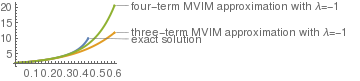
Next we demonstrate the MVIM, which leads to the recurrence:
\[ u_{n+1} = u_n - \int_0^x \left[ e^s \left( u_n (s) - u_{n-1} (s) \right) + e^{-s} \left( u_n^3 (s) - u_{n-1}^3 (s) \right) \right] {\text d}s , \qquad n=1,2,\ldots . \]
With \( u_{-1} =0 , \ u_0 =1 , \) we obtain
\begin{eqnarray*} u_1 (x) &=& 1 - \int_0^x \left[ e^s u_0 (s) + e^{-s} u_0^3 (s) - \cosh s \right] {\text d}s = 1- e^x + \cosh x =1-x - \frac{x^3}{6} - \frac{x^5}{120} - \cdots , \\ u_2 (x) &=& u_1 - \int_0^x \left[ e^s \left( u_1 (s) - u_0 (s) \right) + e^{-s} \left( u_1^3 (s) - u_0^3 (s) \right) \right] {\text d}s = y_2 (x) , \end{eqnarray*}
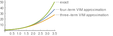
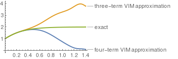
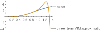
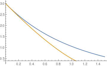
and so on. As we see from the above formulas, we obtain exactly the same sequence of functions, but we performed less calculations. Now we plot the third approximation along with the true solution.
ode1 = {y'[x] + Exp[x]*y[x] + Exp[-x]*(y[x])^3 == Cosh[x], y[0] == 1}
sol = NDSolve[ode1, y, {x, 0, 2}];
Plot[{Callout[y3[x], "three-term VIM approximation"], Callout[y[x] /. sol, "exact"]}, {x, 0, 1}, PlotStyle->Thick]
True solution and MVIM approximations with N = 3 terms.
  1. Abbasbandy S (2007), A new application of He’s variational iteration method for quadratic Riccati differential equation by using Adomian’s polynomials, Journal of Applied Mathematics and Computing, 207:59–63
  2. Tamer A. Abassy, New Applications of the Modified Variational Iteration Method, Studies in Nonlinear Sciences, 2012, Vol. 3, No. 2, pp. 49--61, doi: 10.5829/idosi.sns.2012.3.2.246
  3. Tamer A. Abassy, Magdy A. El-Tawil, and H. El-Zoheiry, Exact solutions of some nonlinear partial differential equations using the variational iteration method linked with Laplace transforms and the Padé technique, Computers and Mathematics with Applications, 2007, Vol. 54, pp. 940--954.
  4. M.A. Fariborzi Araghi, S. Gholizadeh Dogaheh, and Z. Sayadi, The modified variational iteration method for solving linear and nonlinear ordinary differential equations, Australian Journal of Basic and Applied Science, 2011, Vol. 5, No. 10, pp. 406--416.
  5. Inan Ates and Ahmet Yildirim, "Comparison between variational iteration method and homotopy perturbation method for linear and nonlinear partial differential equations with the nonhomogeneous initial conditions," Numerical Methods for Partial Differential Equations, 2010, Vol 26, Issue 6, pp. 1581--1593, doi: https://doi.org/10.1002/num.20511
  6. Elzaki, T.M., Solution of Nonlinear Partial Differential Equations by New Laplace Variational Iteration Method, 2018, doi: 10.5772/intechopen.73291
  7. Ganji D.D. and Sadighi A. (2006) Application of He’s methods to nonlinear coupled systems of reactions. International Journal of Nonlinear Sciences and Numerical Simulation, 2006, Vol, 7, No 4, pp. 411--418.
  8. Ganji DD, Tari H, Jooybari MB (2007) Variational iteration method and homotopy perturbation method for evolution equations. Comput Math Appl 54:1018–1027
  9. Ji-Huan He, "Variational iteration method---a kind of non-linear analytical technique: some examples," International Journal of Non-Linear Mechanics, 1999, Vol 34, 699--708.
  10. Ji-Huan He, "Variational iteration method for autonomous ordinary differential systems," Applied Mathematics and Computation, 2000, Vol. 114, 115--123.
  11. Ameina S. Nuseir and Mohammad Al-Towaiq, The modified variational iteration method for solving the Impenetrable Agar model problem, International Journal of Pure and Applied Mathematics, 2014, Vol. 96, No 4, pp. 445--456, doi: http://dx.doi.org/10.12732/ijpam.v96i4.3
  12. S. S. Samaee, O. Yazdanpanah, and D. D. Ganji, "New approaches to identification of the Lagrange multiplier in the variational iteration method," Journal of the Brazilian Society of Mechanical Sciences and Engineering, 2914, doi: 0.1007/s40430-014-0214-3
  13. Tatari M, Dehghan M (2007), "He’s variational iteration method for computing a control parameter in a semi-linear inverse parabolic equation," Chaos, Solitons & Fractals, 2007, Vol. 33, Issue 2, pp. 671--677.
  14. Tari H., Ganji D.D., and Babazadeh H. (2007) "The application of He’s variational iteration method to nonlinear equations arising in heat transfer," Physics Letters A, Vol. 363, No. 3, pp. 213--217, doi: 10.1016/j.physleta.2006.11.005
  15. Tari H, Ganji D.D., and Rostamian M. (2007) "Approximate solution of K (2, 2), KdV and modified KdV equations by variational iteration method, homotopy perturbation method and homotopy analysis method," International Journal of Nonlinear Sciences and Numerical Simulation, 2007, Vol. 8, pp.203--210.
  16. A.-M. Wazwaz (2009), "The variational iteration method for analytic treatment for linear and nonlinear ODEs," Applied Mathemathics and Computation, 2009, Vol. 212, Issue 1, pp. 120--143.
  17. A.-M. Wazwaz (2006), "A study on linear and nonlinear Schrodinger equations by the variational iteration method," Chaos Solitons Fractals, doi: 10.1016/j.chaos.10.009
  18. A.-M. Wazwaz (2007), The variational iteration method for the exact solution of Laplace equation, Physics Letters A, Vol. 363, No 4, pp. 260--262, doi: 10.1016/j.physleta.2006.11.014
  19. A.-M. Wazwaz (2001) The numerical solution of fifth-order boundary value problems by the decomposition method. Journal of Applied Mathematics and Computing, 136:259–270
  20. A.-M. Wazwaz (2007) The variational iteration method for solving linear and nonlinear systems of PDES, Computers and Mathematics with Applications, 2007, Vol. 54, pp. 895--902.


Complete List of Publications using the Variational Iteration Method


Return to Mathematica page
Return to the main page (APMA0330)
Return to the Part 1 (Plotting)
Return to the Part 2 (First Order ODEs)
Return to the Part 3 (Numerical Methods)
Return to the Part 4 (Second and Higher Order ODEs)
Return to the Part 5 (Series and Recurrences)
Return to the Part 6 (Laplace Transform)
Return to the Part 7 (Boundary Value Problems)