Return to computing page for the first course APMA0330
Return to computing page for the second course APMA0340
Return to computing page for the fourth course APMA0360
Return to Mathematica tutorial for the first course APMA0330
Return to Mathematica tutorial for the second course APMA0340
Return to Mathematica tutorial for the fourth course APMA0360
Return to the main page for the course APMA0330
Return to the main page for the course APMA0340
Return to the main page for the course APMA0360
Return to Part VI of the course APMA0330

Preface


This section provides a stream of examples demonstrating applications of Laplace transformation for solving initial value problems that appear in applications.

Applications


Example 1: If a drag is administrated into the bloodstream in dosages d(t) and is removed at a rate at a rate proportional to the concentration, the concentration c(t) at time t is modeled by the following initial value problem
\[ \frac{{\text d}c}{{\text d}t} = d(t) - k\,c(t), \qquad c(0) =0 , \]
where k > 0 is a positive constant. Suppose that over a 24-hour period, a drag is introduced into the bloodstream at a rate of 24/t0 for exactly t0 hours and then stopped so that
\[ d(t) = \begin{cases} 24/t_0 , & \ 0 \le t \le t_0 , \\ 0, & \ t > t_0 . \end{cases} \]
To model the above piecewise continuous function, Mathematica offers two functions: either
\[ {\bf UnitStep}[x] = \begin{cases} 1, & \ x\ge 0 , \\ 0, & \ x < 0 ; \end{cases} \]
and
\[ {\bf HeavisideTheta}[t] = \begin{cases} 1, & \ t> 0 , \\ 0, & \ t < 0 . \end{cases} \]
The difference between these two functions is what value is assigned at x = 0: UnitStep set its value to 1, while HeavisideTheta leaves it unassigned. The definition of the Heaviside function requires its value at x = 0 to be 1/2. However, for our application of Laplace transform in this example, it does not matter.

Now we solve the corresponding initial value problem with Mathematica. First, we define the input function d(t:

d[t_, t0_] = 24/t0 * UnitStep[t0 - t]
Since the given initial value problem is linear, we can find its explicit solution; here we have two options: either use the Laplace transform or apply the standard command DSolve. So we demonstrate each approach.

Application of Laplace's transform yields an algebraic equation for cL, the Laplace transform of unknown drug concentration:

\[ \lambda\,c^L (\lambda ) = \frac{24}{\lambda\,t_0} \left( 1 - e^{-\lambda\,t_0} \right) - k\,c^L (\lambda ) =0 . \]
Mathematica confirms:
LaplaceTransform[d[t, t0], t, s]
(24 (1 - E^(-s t0)) UnitStep[t0])/(s t0)
Solving for cL, we obtain
\[ c^L (\lambda ) = \frac{1}{\lambda +k} \,\frac{24}{\lambda\,t_0} \left( 1 - e^{-\lambda\,t_0} \right) . \]
The final step is to apply the inverse Laplace transform to the above function. It is convenient to introduce an auxiliary function as the inverse Laplace transform
\[ g(t) = {\cal L}^{-1} \left[ \frac{1}{\lambda (\lambda +k)} \right] = \left( \frac{1}{k} - \frac{1}{k}\, e^{-kt} \right) H(t) \]
because
InverseLaplaceTransform[1/s/(s + k), s, t]
1/k - E^(-k t)/k
As usual, H(t) denotes the Heaviside function
\[ H(t) = \begin{cases} 1, & \ t > 0 , \\ 1/2 , & \ t=0, \\ 0, & \ t < 0 . \end{cases} \]
With this in hand, we find the solution of the given initial value problem explicitly:
\[ c(t) = \frac{24}{t_0} \left[ g(t) - g(t- t_0 ) \right] . \]
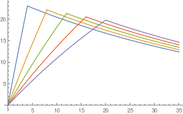
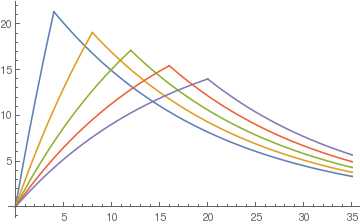
To plot solutions c(t) for different values of parameters k and t0,we use DSolve and and build a table of functions c(t), with 4 hours difference in drug administration, first with k = 0.02 and then k = 0.06.
sol[k_, t0_] := DSolve[{c'[t] == d[t, t0] - k*c[t], c[0] == 0}, c[t], t][[1, 1, 2]]
plotdrug02 = Map[sol[0.02, #] &, {4, 8, 12, 16, 20}]
Plot[plotdrug02, {t, 0, 35}]
plotdrug06 = Map[sol[0.06, #] &, {4, 8, 12, 16, 20}]
Plot[plotdrug06, {t, 0, 35}]
The Laplace transformation can be successfully applied to solve an integral equation of a convolution type (also known as the Volterra integral equation):
\begin{equation} \label{EqApp.1} y(t) = f(t) + \int_0^t K(t- \tau )\,y(\tau )\,{\text d}\tau , \end{equation}
where the function f(t) and the kernel function K(Θ) are known, while y(t) is unknown. Since the integral in \eqref{EqApp.1} is the convolution of the kernel function K(Θ) and the unknown function y(t), application of the Laplace transform yields
\begin{equation} \label{EqApp.2} y^L = f^L + K^L y^L , \qquad \mbox{where} \quad y^L = {\cal L} \left[ y(t) \right] = \int_0^{\infty} y(t)\,e^{-\lambda t} {\text d}t . \end{equation}
This equation can be immediately solved and the inverse Laplace transformation provides the solution:
\begin{equation} \label{EqApp.3} y(t) = {\cal L}^{-1} \left[ \frac{1}{1 - K^L (\lambda )}\, f^L (\lambda ) \right] (t) . \end{equation}
Example 2: The problem of finding the curve down which a bead placed anywhere will fall to the bottom in the same amount of time is called the tautochrone problem. It was first solved by Christiaan Huygens in 1659, who proved that such curve must be a cycloid. The name of such curve stems from the Greek tauto, meaning ``same,'' and chronos (χρονος), meaning ``time.'' Following Niels Abel, we formulate the problem in integral form.
Tautochrone curve.
Let (x,y) be the position of the bead at some intermediate time before it reaches the origin. Let s denote the arc length along the curve measured from the origin to (x,y). According to the principle of conservation of energy, the gain in kinetic energy of the bead must equal its loss of potential energy in falling from some fixed point (x0,y0) to (x,y). Therefore, we get \[ \frac{1}{2}\,mv^2 = mg (y_0 -y). \] Since v = ds/dt is the velocity, we have \[ \frac{{\text d}s}{{\text d}t} = -\sqrt{2g} \,\sqrt{y_0 - y} , \qquad\mbox{or}\qquad \frac{{\text d}s}{\sqrt{y_0 - y}} = - \sqrt{2g} \,{\text d}t , \] where the minus sign indicates that s is decreasing with increasing t. Assuming that the arc length s is some yet unknown function of y (namely, s = f(y)), we derive the differential equation \[ \frac{f' (y) \,{\text d}y}{\sqrt{y_0 - y}} = - \sqrt{2g} \,{\text d}t . \]
After integration over the (constant) duration T0 of descent, we obtain \[ \int_0^{y_0} \frac{f' (y) \,{\text d}y}{\sqrt{y_0 - y}} = -\sqrt{2g} \,\int_{T_0}^0 \,{\text d}t \qquad\mbox{or} \qquad T_0 = \frac{1}{\sqrt{2g}} \int_0^{y_0} \frac{f' (y) \,{\text d}y}{\sqrt{y_0 - y}} . \] We can rewrite the latter equation as a convolution of the functions y-1/2 and f'(y): \[ T_0 = \frac{1}{\sqrt{2g}} \, y^{-1/2} \ast f' . \] With the aid of the Laplace transform, we easily solve the convolution equation to obtain \[ {\cal L} [T_0 ] = \frac{1}{\sqrt{2g}} \,{\cal L} \left[ y^{-1/2} \right] \cdot {\cal L} [f' ] \qquad\Longrightarrow\qquad {\cal L} [f' ] = \sqrt{\frac{2g}{\pi}} \,T_0 \,\lambda^{-1/2} , \] because \( {\cal L} [y^{-1/2} ] = \sqrt{\pi / \lambda} \) and \( {\cal L} [T_0 ] = T_0 /\lambda \) (see formula in Table). Note that the Laplace transformation is taken with respect to the variable y. Thus, \[ f' (y) = \frac{{\text d}s}{{\text d}y} = \sqrt{1 + \left( \frac{{\text d}x}{{\text d}y} \right)^2} = \frac{\sqrt{2g}}{\pi} \,T_0 \,y^{-1/2} . \] Setting \( k=(2gT_0^2 )/\pi^2 , \) we obtain the equation: \[ \frac{{\text d}x}{{\text d}y} = \sqrt{\frac{k-y}{y}} . \] After the substitution \[ y = k\,\sin^2 \frac{\theta}{2} \qquad \mbox{and} \qquad {\text d}x = k\,\cos^2 \frac{\theta}{2}\,{\text d}\theta , \] it becomes \[ x= k\int \cos^2 \frac{\theta}{2}\,{\text d}\theta = \frac{k}{2} \int (1+ \cos\theta )\,{\text d}\theta = \frac{k}{2}\, (\theta + \sin\theta ) +C . \] We set the constant of integration C to zero because the curve must pass through the origin, and y=0 when θ=0. Finally, \[ x= \frac{k}{2}\, (\theta + \sin\theta ) , \qquad y =\frac{k}{2}\, (1-\cos\theta ) . \] This curve is known as the cycloid.    ■
Example 3: Let us consider a boundary value problem
\[ y'' + 2\,y' + 5\,y = 0 \qquad (0 < x < \ell ), \qquad y(0) =1, \quad y' (\ell ) = 0. \tag{3.1} \]
We apply the Laplace transformation to the given differential equation and obtain
\[ \lambda^2 y^L (\lambda ) - y' (0) - \lambda + 2\lambda\, y^L - 2 + 5\,y^L = 0. \]
Since we don't know the value of the derivative of the unknown function y(x) at the leftend x = 0, we denote it by \( y' (0) = c . \) Then the Laplace transform of the required function y(x) is
\[ y^L (\lambda ) = {\cal L} \left[ y(t) \right] (\lambda ) = \int_0^{\infty} y(x)\, e^{-\lambda x} {\text d}x = \frac{\lambda + c +2}{\lambda^2 + 2\lambda + 5} . \]
Application of the inverse Laplace transform to this function yields
\[ y(x) = {\cal L}^{-1} \left[ \frac{\lambda + c +2}{\lambda^2 + 2\lambda + 5} \right] = \left( c+2 \right)e^{-x} \sin x\,\cos x + \frac{1}{2}\, e^{-x} \left( 2\cos 2x - \sin 2x \right) , \tag{3.2} \]
InverseLaplaceTransform[(1)/(s^2 + 2*s + 5), s, t];
Simplify[Assuming[t > 0, ComplexExpand[%]]]
E^-t Cos[t] Sin[t]
InverseLaplaceTransform[(s)/(s^2 + 2*s + 5), s, t];
Simplify[Assuming[t > 0, ComplexExpand[%]]]
1/2 E^-t (2 Cos[2 t] - Sin[2 t])
To satisfy the boundary condition at x = ℓ, we set
\[ 2 e^{\ell}\,y' (\ell ) = \left( c+2 \right) \left[ 2\cos 2\ell - \sin 2\ell \right] -4\,\cos 2\ell - 3\,\sin 2\ell . \]
y[t_] = 1/2 E^-t (2 Cos[2 t] - Sin[2 t]) + K* E^-t Cos[t] Sin[t];
Simplify[D[y[t], t]]2*Exp[t]
2 (-2 + K) Cos[2 t] - (3 + K) Sin[2 t]
Equating the latter to zero, we obtain the equation for determinantion of parameter c:
\[ c = -2 + \frac{4\,\cos 2\ell + 3\,\sin 2\ell}{2\cos 2\ell - \sin 2\ell} . \]
   ■
Example 4: 
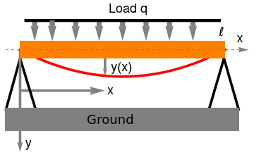
A uniformly loaded beam of length ℓ is supported at both ends. The deflection y(x) is a function of horizontal position x and obeys the differential equation
\[ \frac{{\text d}^4 y(x)}{{\text d}x^4} = \frac{1}{E\,I}\,q(x) , \tag{4.1} \]
where E is Young’s modulus, I is the moment of inertia and q(x) is the load per unit length at point x. We assume in this problem that q(x) = q (a constant). The boundary conditions are (i) no deflection at x = 0 and x = ℓ; (ii) no curvature of the beam at x = 0 and x = ℓ.
line1 = Graphics[{Black, Thickness[0.01], Line[{{-1.99, -1.02}, {-1.749, -0.15}, {-1.49, -1}}]}];
line2 = Graphics[{Black, Thickness[0.01], Line[{{1.98, -1.02}, {1.73, -0.15}, {1.48, -1}}]}];
box = Graphics[{Orange, Rectangle[{1.75, 0.15}, {-1.75, -0.15}]}];
box2 = Graphics[{Gray, Rectangle[{-2, -1.4}, {2.0, -1}]}];
s = Plot[0.15*(x^2 - 1.75^2), {x, -1.75, 1.75}, PlotStyle -> {Thickness[0.01], Red}, AspectRatio -> 1/3];
rod = Graphics[{Black, Thickness[0.012], Line[{{-1.65, 0.5}, {1.65, 0.5}}]}];
arrow = Graphics[{Gray, Dashed, Arrowheads[0.04], Arrow[{{-2, 0}, {2.15, 0}}]}];
aa = Graphics[{Gray, Thickness[0.01], Arrowheads[0.03], Arrow[{{-0.3, 0.0}, {-0.3, -0.45}}]}];
aay = Graphics[{Gray, Thickness[0.01], Arrowheads[0.04], Arrow[{{-1.75, 0.0}, {-1.75, -1.75}}]}] t1 = Graphics[{Black, Text[Style["y(x)", 18], {-0.01, -0.3}]}];
t2 = Graphics[{Black, Text[Style["y", 18], {-1.6, -1.6}]}];
t3 = Graphics[{Black, Text[Style["Ground", 18, FontFamily -> "Mathematica1"], {-0.2, -1.2}]}];
t4 = Graphics[{Black, Text[Style["\[ScriptL]", 18, FontFamily -> "Mathematica1"], {1.7, 0.3}]}];
tx = Graphics[{Black, Text[Style["x", 18], {2.01, 0.2}]}];
txx = Graphics[{Black, Text[Style["x", 18], {-0.2, -0.7}]}];
ar1 = Graphics[{Gray, Thickness[0.02], Arrowheads[0.06], Arrow[{{-1.6, 0.5}, {-1.6, 0.15}}]}];
r2 = Graphics[{Gray, Thickness[0.02], Arrowheads[0.06], Arrow[{{-1.2, 0.5}, {-1.2, 0.15}}]}];
ar3 = Graphics[{Gray, Thickness[0.02], Arrowheads[0.06], Arrow[{{-0.8, 0.5}, {-0.8, 0.15}}]}];
ar4 = Graphics[{Gray, Thickness[0.02], Arrowheads[0.06], Arrow[{{-0.4, 0.5}, {-0.4, 0.15}}]}];
ar5 = Graphics[{Gray, Thickness[0.02], Arrowheads[0.06], Arrow[{{0.0, 0.5}, {0.0, 0.15}}]}];
ar6 = Graphics[{Gray, Thickness[0.02], Arrowheads[0.06], Arrow[{{0.4, 0.5}, {0.4, 0.15}}]}];
ar7 = Graphics[{Gray, Thickness[0.02], Arrowheads[0.06], Arrow[{{0.8, 0.5}, {0.8, 0.15}}]}];
ar8 = Graphics[{Gray, Thickness[0.02], Arrowheads[0.06], Arrow[{{1.2, 0.5}, {1.2, 0.15}}]}];
ar9 = Graphics[{Gray, Thickness[0.01], Arrowheads[0.06], Arrow[{{-1.75, -0.7}, {-0.3, -0.7}}]}];
Show[ar1, ar2, ar3, ar4, ar5, ar6, ar7, ar8, ar9, line1, line2, aa, aay, s, rod, box, box2, t1, t2, tx, txx, t3, t4, arrow, ar2, t5]
Beam load
In addition to being subject to a uniformly distributed load, a beam is supported so that there is no deflection and no curvature of the beam at its ends. Since the curvature of the function y(x) is
\[ \kappa = \frac{\left\vert y'' (x) \right\vert}{\left( 1 + y'^{2} \right)^{3/2}} , \]
we come to the following boundary conditions
\[ y(0) = 0, \quad \left. \frac{{\text d}^2 y}{{\text d}x^2} \right\vert_{x=0} = 0, \qquad y(\ell ) = 0, \quad y'' (\ell ) = 0 . \tag{4.2} \]
Applying a Laplace transform to the differential equation (4.1), we find that the Laplace transform of the deflection, yL, satisfies the algebraic equation
\[ \lambda^4 y^L - y'''(0) - \lambda^2 y' (0) = \frac{q}{E\,I}\,\frac{1}{\lambda} . \]
Solving the latter, we obtain an explicit formula for yL:
\[ y^L (\lambda ) = \int_0^{\infty} y(t)\, e^{-\lambda t} {\text d}t = \frac{y'''(0)}{\lambda^4} + \frac{y' (0)}{\lambda^2} + \frac{q}{E\,I}\,\frac{1}{\lambda^5} . \tag{4.3} \]
Applying the inverse Laplace transform and using the formula
\[ {\cal L}^{-1} \left[ \frac{1}{\lambda^n} \right] = \frac{x^{n-1}}{(n-1)!} , \]
we determine the deflection of the beam
\[ y(x) = \frac{q}{E\,I}\,\frac{x^4}{24} + y' (0) \,x + \frac{y'''(0)}{6}\, x^3 . \]
The derivatives evaluated at the origin are unknown constants, but they can be determined by using the remaining two boundary conditions (4.2) at x = ℓ. Hence, we get two equations for their determination:
\begin{align*} y(\ell ) &= \frac{q}{E\,I}\,\frac{\ell^4}{24} + y' (0) \,\ell + \frac{y'''(0)}{6}\, \ell^3 = 0, \\ y'' (\ell ) &= \frac{q}{E\,I}\,\frac{\ell^2}{2} + y'''(0)\,\ell = 0. \end{align*}
We ask mathematica to solve this system of algebraic equations.
Solve[{q*L^4/24 + x1*L + x3*L^3/6 == 0, q*L^2/2 + x3*L == 0}, {x1, x3}]
{{x1 -> (L^3 q)/24, x3 -> -((L q)/2)}}
Finally substituting the values of these derivatives gives the formula for y(x):
\[ y(x) = \frac{q}{E\,I} \left[ \frac{x^4}{24} - \frac{\ell}{12}\, x^3 + \frac{\ell^3}{24}\,x \right] . \]
   ■
Example 5: The principle of financial Ponzi scheme is to attract potential inverters promissing high rate of return, which is impossible to deliver. The only way this financial piramid can work is when new investement will be sufficient to pay the promised interest. This financial scheme was carried out from 1869 to 1872 by Adele Spitzeder in Germany and by Sarah Howe in the United States in the 1880s through the "Ladies' Deposit".

In the 1920s, Charles Ponzi (1882--1949) carried out this piramid and became well known throughout the United States because of the huge amount of money that he took in. His original scheme was based on the legitimate arbitrage of international reply coupons for postage stamps, but he soon began diverting new investors' money to make payments to earlier investors and to himself. Recent example of this financial piramod provides the Chara bank operated more than a year in Moscow (Russia). However, the largest Ponzi scheme operated in the United States, where its owner, Bernard Madoff, was arrested in 2008 for allegedly running a multigillion-dollar that caused a lost of $50 billion dollars in investments. Mardoff's fund offered 10% return for investors, while Chara bank paid about 20%.

We present a mathematical model following
Artzrouni, M., The mathematics of Ponzi schemes, Mathematical Social Sciences, 2009, pp. 190--201.

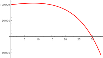
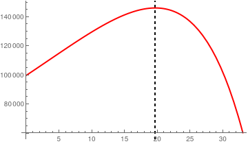
Assume that the fund starts at t = 0 with an initial deposite K ≥ 0 followed bya continuous cash inflow s(t). Let us denote by rp a promised rate of return and by rn a nominal interest rate corresponding to the market value. We consider the case when rp > rn, thw fund oromised moew than it can deliver. The promised rate rp may be called the "Ponzi rate" and is equal to 0.10 in Madoff's case when ewalistic rate was 0.02.

To attract investors, all Ponzi scheme followers offered customers a possibility to withdraw the interest. For simplicity, we assume that the withdrawal rate rw is constant. Then initial investors expect to gain (according to continuous compound interest) the amount \( \displaystyle K\, e^{t \left( r_p - r_w \right)} \) in accumilated capital at time t.

Withdrawals by those who added to the Ponzi fund between times 0 and t are obtained by calculating withdrawals for those who invested at time u and then summing for u between 0 and t. The quantity s( u) is invested at time u with an expected growth rate rprw for the duration tu. The expected accumilated value at time t is then \( \displaystyle s(u)\, e^{\left( r_p - r_w \right) (t-u)} {\text d} u . \) The density of withdrawals at time t is then \( \displaystyle r_u s(u)\, e^{\left( r_p - r_w \right) (t-u)} \) with a sum \( \displaystyle r_u \int_0^t s(u)\,e^{\left( r_p - r_w \right) (t-u)} {\text d} u \) of withdrawals W(t) is then the sum of withdrawals by initial investors and by those who invested between times 0 and t:

\[ W(t) = r_w \left( K\, e^{t \left( r_p - r_w \right)} + \int_0^t s(u)\, e^{\left( r_p - r_w \right) (t-u)} {\text d} u \right) . \tag{5.1} \]
If S(t) is the ampount in the fund at time t, then S(t+dt) is obtained by adding to S(t) the nominal interest rnS(t), the inflow of fresh money s(t)dt and subtracting the withdrawals W(t)dt:
\[ S(t + {\text d}t) = S(t) + {\text d} t \left[ r_n S(t) + s(t) - W(t) \right] \]
For dt → 0, the amount S(t) is the solution to the initial value problem for the first order linear differential equation
\[ \frac{{\text d} S(t)}{{\text d} t} = r_n S(t) + s(t) - W(t) . \qquad S(0) = C , \tag{5.2} \]
where C is the initial value, which may or may not be equal to K, the initial deposit made by customers.

A simple model for inflow investment is the Malthus law:

\[ s(t) = s_0 e^{r_i t} , \]
wheres0 is the initial density of the deposits and ri is the investment (malthus) rate. The integral in Eq.(5.1) is the convolution of two functions:
\[ \int_0^t s(u)\, e^{\left( r_p - r_w \right) (t-u)} {\text d} u = s \star \left( e^{\left( r_p - r_w \right) t} \right) . \]
Applying the Laplace transform to the convolution integral, we get
\[ {\cal L} \left[ s \star \left( e^{\left( r_p - r_w \right) t} \right) \right] = s^L \cdot \frac{1}{\lambda - \left( r_p - r_w \right)} , \]
where
\[ s^L = {\cal L} \left[ s (t) \right] = \int_0^{\infty} s(t)\, e^{-\lambda t} {\text d} t = \frac{s_0}{\lambda - r_i} \]
is the Laplace transform of s(t). As usual, we denote by SL the Laplace transform of the amount of the fund, we obtain from the initial value problem (5.2) a linear equation:
\[ \lambda\,S^L - C = r_n S^L + \frac{s_0}{\lambda - r_i} - \frac{r_w K}{ \lambda - \left( r_p - r_w \right)} - \frac{r_w s_0}{\lambda - r_i} \cdot \frac{1}{\lambda - \left( r_p - r_w \right)} . \]
Solving this equation, we get
\[ S^L (\lambda ) = \frac{C}{\lambda - r_n} + \frac{s_0}{\left( \lambda - r_n \right) \left( \lambda - r_m \right)} - \frac{1}{\lambda - r_n} \cdot \frac{r_w K}{\lambda - \left( r_p - r_w \right)} - \frac{r_w s_0}{\left( \lambda - r_m \right) \left( \lambda - r_n \right)} \cdot \frac{1}{\lambda - \left( r_p - r_w \right)} . \tag{5.3} \]
Using the relations of the inverse Laplace transform
\begin{align*} {\cal L}^{-1} \left[ \frac{1}{\lambda -a} \right] &= e^{at} H(t) , \\ {\cal L}^{-1} \left[ \frac{1}{\left( \lambda -a \right) \left( \lambda - b \right)} \right] &= \frac{1}{a-b} \left[ e^{at} - e^{bt} \right] H(t) , \\ {\cal L}^{-1} \left[ \frac{1}{\left( \lambda -a \right) \left( \lambda - b \right)\left( \lambda - c \right)} \right] &= \frac{e^{at}}{\left( a - b \right)\left( a - c \right)} - \frac{e^{bt}}{\left( a - b \right)\left( b - c \right)} + \frac{e^{ct}}{\left( a - c \right)\left( b - c \right)} , \end{align*}
we find the explicit expression for S(t):
InverseLaplaceTransform[1/(s - a), s, t]
InverseLaplaceTransform[1/(s - a)/(s - b), s, t]
(E^(a t) - E^(b t))/(a - b)
InverseLaplaceTransform[1/(s - a)/(s - b)/(s - c), s, t]
E^(a t)/((a - b) (a - c)) - E^(b t)/((a - b) (b - c)) - E^( c t)/((a - c) (-b + c))
\begin{align*} S(t) &= C\, e^{r_m t} + \frac{s_0}{r_m - r_n} \left( e^{r_m t} - e^{r_n t} \right) - \frac{r_w K}{r_p - r_w - r_n} \left( e^{(r_p - r_w )t} - e^{r_n t} \right) \\ & \quad - \frac{r_w s_0}{\left( r_m - r_n \right) \left( r_m - r_p + r_w \right)} \, e^{r_m t} + \frac{r_w s_0}{ \left( r_m - r_n \right) \left( r_n - r_p + r_w \right)}\, e^{r_n t} - \frac{r_w s_0}{\left( r_m - r_p + r_w \right) \left( r_n - r_p + r_w \right)} \, e^{\left( r_p - r_w \right) t} . \end{align*}
      We plot the amount in the fund S(t) at time t

soln = With[{K = 100000, rn = .02, rw = .01, rp = .1, ri = 0.15, s0 = 1}, Solve[\[Lambda] SL - K == rn SL + s0/(\[Lambda] - ri) - rw (K/(\[Lambda] - rp + rw) + s0/(\[Lambda] - ri)*1/(\[Lambda] - rp + rw)), SL]] // FullSimplify
S[t_] = InverseLaplaceTransform[( 1499.9000000000003` + \[Lambda] (-24999.` + 100000.` \[Lambda]))/((-0.15` + \[Lambda]) \ (-0.09000000000000001` + \[Lambda]) (-0.02` + \[Lambda])), \[Lambda], t]
Plot[S[t], {t, 0, 33}, PlotStyle -> {Red, Thick}]
       Ponzi investment.            Mathematica code

Tipping Point is at maximum of S
t/. Last[FindMaximum[S[t], {t, 2}]]
19.6592
S[20]
146220.
      We plot S(t)
Plot[S[t], {t, 0, 33}, PlotStyle -> {Red, Thick}, GridLines -> {{t /. Last[FindMaximum[S[t], {t, 2}]]}, None}, GridLinesStyle -> Directive[Black, Thick, Dashed]]

Now we plot with Manipulation option:
Clear[Cap, K, t, u, S, s, rp, rn, rw, ri, W];
mani1 = Manipulate[ S = InverseLaplaceTransform[ With[{s0 = 1}, Solve[\[Lambda] SL - K == rn SL + s0/(\[Lambda] - ri) - rw (K/(\[Lambda] - rp + rw) + s0/(\[Lambda] - ri)*1/(\[Lambda] - rp + rw)), SL]][[1, 1, 2]], \[Lambda], t]; max = t /. Last[FindMaximum[S, {t, 2}]]; pltS = Plot[S, {t, 0, 33}, PlotLabel -> "Tipping Point= " <> ToString[max] <> " periods", Axes -> False, Frame -> {True, True, False, False}, GridLines -> {{max}, None}, GridLinesStyle -> Directive[Black, Thick, Dashed], PlotStyle -> Red, FrameLabel -> {{"Balance in Fund", None}, {"Time \[LongRightArrow]", None}}]; arr1 = Graphics[Arrow[{{max - 1, K}, {max - 5, K}}]]; arr2 = Graphics[Arrow[{{max + 1, K}, {max + 5, K}}]]; Show[pltS, arr1, arr2, Epilog -> {Text["Legal", {max - 3, K + 500}], Text["Illegal", {max + 3, K + 500}]}], (*controls*) {{K, 10001, "Initial Capital"}, 10001, 100001, 10000, Appearance -> "Labeled"}, {{rn, .04, "Actual earnings rate"}, .02, .06, Appearance -> "Labeled"}, {{rw, .01, "Withdrawal rate"}, .01, .12, Appearance -> "Labeled"}, {{rp, .10, "Promised earnings rate"}, .07, .12, Appearance -> "Labeled"}, {{ri, 0.15, "Investment rate"}, .05, .2, Appearance -> "Labeled"} ]
End of Example 5
   ■


  1. Armenti, A., The Physics of Sports, 1992, AIP-Press, New York, 978-0-88318-946-7
  2. Lisa, M., The Physics of Sports, 2016, ISBN13: 9780073513973
  3. Laws, K. and Sugano, A., Physics and the Art of Dance: Understanding Movement, 2nd Edition, 2008, Oxford University Press, ISBN-13: 978-0195341010
  4. Kim, H. and Elzaki, T.M., The Representation on Solutions of Burger’s Equation by Laplace Transform, Int. Journal of Math. Analysis, 2014, Vol. 8, No. 31, 1543 - 1548; http://dx.doi.org/10.12988/ijma.2014.46185
  5. The Physics of Sports, Real world physics problems.


Return to Mathematica page
Return to the main page (APMA0330)
Return to the Part 1 (Plotting)
Return to the Part 2 (First Order ODEs)
Return to the Part 3 (Numerical Methods)
Return to the Part 4 (Second and Higher Order ODEs)
Return to the Part 5 (Series and Recurrences)
Return to the Part 6 (Laplace Transform)
Return to the Part 7 (Boundary Value Problems)