Part I: Plotting
This tutorial contains many Mathematica scripts. You, as the user, are free to use all codes for your needs, and have the right to distribute this tutorial and refer to this tutorial as long as this tutorial is accredited appropriately. I would like to extend my gratitude to all of the students that aided me in developing this tutorial. The coding, testing, and debugging required a concerted effort, and the following students deserve recognition for their input: Emmet and Jesse Golden-Marx (Fall 2011), Pawel Golyski (Fall 2012). Any comments and/or contributions for this tutorial are welcome; you can send your remarks to <Vladimir_Dobrushkin@brown.edu>
Return to computing page for the second course APMA0340
Return to Mathematica tutorial page for the first course
Return to Mathematica tutorial page for the second course
Return to the main page for the course APMA0330
Return to the main page for the course APMA0340
1.1. Plotting functions
One of the best characteristics of Mathematica is its plotting ability. It is very easy to plot a variety of functions using Mathematica. For a plot, it is necessary to define the independent variable that you are graphing with respect to. Mathematica automatically adjusts the range over which you are graphing the function.
This is a simple Plot command. In this example, we are just plotting a function using Mathematica default capabilities, but it is possible to specify the range with PlotRange command. The above graph can also be obtained with the following script:
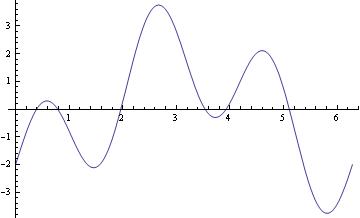
Plot[2*Sin[3*x]-2*Cos[x], {x,0,2Pi}, PlotRange -> Automatic]
Epilog -> {Text[Style["hello", 25], Scaled[{0.5, 0.5}], #], Red, Point@{.5, .5}},
PlotLabel -> ToString@#] & /@ {{-2.5, 0}, {2.5, 0}, {0, -2}, {0, 2}, {2, 2}, {-3, -2}}
 |
 |
 |
 |
 |
 |
Epilog -> {Text[Style["hello", 25], Scaled[{0.5, 0.5}], #], Red, Point@{.5, .5}},
PlotLabel -> ToString@#] & /@ {{-2.5, 0}, {2.5, 0}, {0, -2}, {0, 2}, {2, 2}, {-3, -2}}
 |
 |
 |
 |
 |
 |
http://reference.wolfram.com/language/howto/AddTextToAGraphic.html.en
To add test outside the picture, see
http://reference.wolfram.com/language/howto/AddTextOutsideThePlotArea.html.en
The general reference is
http://reference.wolfram.com/language/howto/AddTextToAGraphic.html
On most computer systems, Mathematica can produce not only graphics but also sound. Mathematica treats graphics and sound in a closely analogous way, using command Play. For instance, the previous function can be used to play, on a suitable computer system, a pure tone with a frequency of 440/2π hertz for one second.
For multiple plots, use either command Show or you can use {} with commas. Show can be used to change the options of an existing graphic or to combine multiple graphics.

Show[{g1, Graphics[Circle[]]}, Background -> Yellow, AspectRatio -> Automatic]

A graphic of a function can be made discrete:
Point[Table[{x, Sin[x] - 1/3 Cos[3 x]}, {x, 0, 6, .2}]]}, Axes -> True]

g1[0]
Show[bp, AxesOrigin -> {0, -1/3}, AxesLabel -> {"x", "y"}]

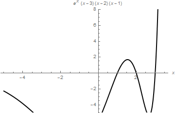
When you need to restrict the vertical range, use PlotRange command as the following example shows.
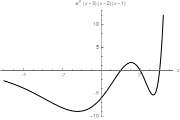
AxesLabel -> {x, (x - 1)*(x - 2)*(x - 3)*Exp[x]}]
PlotStyle -> {Black, Thick}, AxesLabel -> {x, (x - 1)*(x - 2)*(x - 3)*Exp[x]}]
 |
 |
Plot sine function downward:
ListLinePlot[data1, PlotRange -> All];
ticks = Table[{-x, x}, {x, -5, 5, .2}];
ListLinePlot[{#, -#2} & @@@ data1, PlotRange -> {All, 1}, Ticks -> {All, ticks}, Axes -> True, PlotStyle -> Thick]

ListLinePlot[data1, PlotRange -> All];
ticks = Table[{-x, x}, {x, -5, 5, .2}];
ListLinePlot[{#, -#2} & @@@ data1, PlotRange -> {-1.3, 1.3},
Ticks -> {All, ticks}, Frame -> False, PlotRange -> All,
Epilog -> {Text["x", {5.5, 0}], Text["y", {0, -1.4}]},
PlotRangeClipping -> False, ImagePadding -> {{20, 20}, {20, 20}}]

Now plot with arrows, but without units:
Graphics[Join[{Arrowheads[a]},
Arrow[{{0, 0}, #}] & /@ {{x, 0}, {0, y}}, {Text[
Style["x", FontSize -> Scaled[f]], {0.95*x, 0.1*y}],
Text[Style["y", FontSize -> Scaled[f]], {0.1 x, 1*y}]}]]
ListLinePlot[data1, PlotRange -> All];
ticks = Table[{-x, x}, {x, -5, 5, .2}];
Show[ListLinePlot[{#, -#2} & @@@ data1, PlotRange -> {-1.3, 0},
Ticks -> {None, None}, Frame -> False, PlotRange -> All,
PlotRangeClipping -> False, ImagePadding -> {{20, 20}, {20, 20}}],
axes[5.3, -1.33, .06, .05], Axes -> False]

Example. Tractrix (from the Latin verb "trahere" -- pull, drag; plural: tractrices) is the curve along which an object moves, under the influence of friction, when pulled on a horizontal plane by a line segment attached to a tractor (pulling) point that moves at a right angle to the initial line between the object and the puller at an infinitesimal speed. By associating the object with a dog, the string with a leash, and the pull along a horizontal line with the dog's master, the curve has the descriptive name hundkurve (dog curve) in German. It is therefore a curve of pursuit. It was first introduced by Claude Perrault (1613 -- 1688) in 1670. Trained as a physician, Claude was invited in 1666 to become a founding member of the French Academie des Sciences, where he earned a reputation as an anatomist. The first known solution was given by Christian Huygens (1692), who also named the curve the tractrix. Its parametric equation is
To plot tractrix curve, we use the following code:
Manipulate[
ParametricPlot[tractrix[a][t] // Evaluate, {t, 0, .99*\[Pi]},
PlotRange -> {0, 7}], {a, 1, 6}]
Export["tractrix1.gif",%]

Plot[y'[x] = -Sqrt[a^2 - x^2]/x, {x, 0, 20},
PlotRange -> {-10, 10}], {a, 0, 20}]

a Log[x] + a Log[a^2 + a Sqrt[a^2 - x^2]]]}}
Plot[-Sqrt[a^2 - x^2] + a Log[a] - a Log[a^2] - a Log[x] + a Log[a^2 + a Sqrt[a^2 - x^2]], {x, 0, 20}, PlotRange -> All], {a, 1, 20}]

Discontinuous Functions
Direction Fields
Implicit Plot
Parametric Plot
Labeling Figures
Figures with Arrows
Electric circuits
Plotting with Filling
Polar Plots
Some Famous Curves
Cycloids
Return to Mathematica page
Return to the main page (APMA0330)
Return to the Part 2 (First Order ODEs)
Return to the Part 3 (Numerical Methods)
Return to the Part 4 (Second and Higher Order ODEs)
Return to the Part 5 (Series and Recurrences)
Return to the Part 6 (Laplace Transform)
Return to the Part 7 (Boundary Value Problems)