Preface
This is a tutorial made solely for the purpose of education and it was designed for students taking Applied Math 0330. It is primarily for students who have very little experience or have never used Mathematica before and would like to learn more of the basics for this computer algebra system. As a friendly reminder, don't forget to clear variables in use and/or the kernel.
Finally, the commands in this tutorial are all written in bold black font, while Mathematica output is in regular fonts. This means that you can copy and paste all commands into Mathematica, change the parameters and run them. You, as the user, are free to use the scripts to your needs for learning how to use the Mathematica program, and have the right to distribute this tutorial and refer to this tutorial as long as this tutorial is accredited appropriately.
Finally, the commands in this tutorial are all written in bold black font, while Mathematica output is in normal font. This means that you can copy and paste all commands into Mathematica, change the parameters and run them. You, as the user, are free to use the scripts for your needs to learn the Mathematica program, and have the right to distribute this tutorial and refer to this tutorial as long as this tutorial is accredited appropriately.
Return to computing page for the second course APMA0340
Return to Mathematica tutorial for the second course APMA0330
Return to Mathematica tutorial for the first course APMA0340
Return to the main page for the course APMA0340
Return to the main page for the course APMA0330
Return to Part IV of the course APMA0330
Numerical Solutions
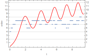
The order of a numerical method used in NDSolve is a variable. Based on [[make brown]]What's inside InterpolatingFunction[{{1., 4.}}, <>]?,[[end brown]] the following shows the order at each step. Note that the first few steps are NDSolve getting its bearings before the first Adams steps (order 4). With InterpolationOrder -> All, the solution is returned with local series for the Adams steps. Their length should be one more than the order of the step, I think. The documentation says it should be the "same order as the underlying method used."
Example. let use Adams method to solve numerically the following initial value problem
Method -> "Adams", InterpolationOrder -> All];
adamsifn = x /. First@adamssol
(*ifn[[4]]= local series coefficients*)
Transpose@{Flatten@adamsifn["Grid"],
Rescale[#, MinMax[#], {0, 12}] &@adamsifn["ValuesOnGrid"]}}, Joined -> {False, True},
Frame -> True, FrameLabel -> {"t", "order"}, FrameTicks -> {Automatic, Range@12},
GridLines -> {None, Automatic}, PlotStyle -> {Thick, Red}]
1.4.7. Numerical Solutions of Second Order ODEs
Example 1.4.3:
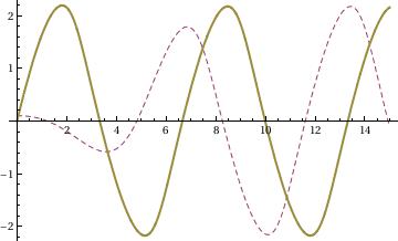
Rayleigh's equation is a non-linear equation
\[ x'' + \mu \left( x^2 -1\right) x +x =0 , \]
that arises in the study of the motion of a violin string. We plot three solutions subject to three different initial conditions:
x'[0] == 0}, x[t], {t, 0, 15}]
Plot[Evaluate[x[t] /. {numsol, numsol2, numsol3}], {t, 0, 15},
PlotStyle -> {GrayLevel[0.1], Dashed, Thick}]
To identify each graph, it is helpful to use PlotLegend option:
PlotLegends -> Automatic]

PlotLegends -> {"IC: x(0)=1, x'(0)=0", "IC: x(0)=0.1, x'(0)=0", "IC: x(0)=0, x'(0)=2"}]

Return to Mathematica page
Return to the main page (APMA0330)
Return to the Part 1 (Plotting)
Return to the Part 2 (First Order ODEs)
Return to the Part 3 (Numerical Methods)
Return to the Part 4 (Second and Higher Order ODEs)
Return to the Part 5 (Series and Recurrences)
Return to the Part 6 (Laplace Transform)