Preface

---

This is a tutorial made solely for the purpose of education and it was designed for students taking Applied Math 0330. It is primarily for students who have very little experience or have never used Mathematica before and would like to learn more of the basics for this computer algebra system. As a friendly reminder, don't forget to clear variables in use and/or the kernel.

Finally, the commands in this tutorial are all written in bold black font, while Mathematica output is in normal font. This means that you can copy and paste all commands into Mathematica, change the parameters and run them. You, as the user, are free to use the scripts for your needs to learn the Mathematica program, and have the right to distribute this tutorial and refer to this tutorial as long as this tutorial is accredited appropriately.

Fundamental Sets of Solutions

---

A set of m functions \( \left\{ f_1 (x), \ f_2 (x), \ \ldots , \ f_m (x) \right\} , \) each defined and continuous on some interval \( |a, b| , \quad a < b, \) is said to be linearly dependent on this interval if there exist constants \( k_1 , k_2 , \ldots , k_m \) not all of them zero, such that

for every x in the interval |a,b|. Otherwise, the functions \( \left\{ f_1 (x), \ f_2 (x), \ \ldots , \ f_m (x) \right\} , \) are said to be linearly independent. Two functions f and g are linearly dependent if and only if one of them is a constant multiple of another. ■

A set of functions \( \left\{ f_1 , \ f_2 , \ \ldots , \ f_m \right\} \) is linearly dependent on an interval if at least one of these functions can be expressed as a linear combination of the remaining functions (with at least one nonzero coefficient). The interval on which functions are defined plays a crucial role in this definition: the set of functions can be linearly independent on some interval, but can become dependent on another one (see next example).

Example: Depedence on the interval

Any set \( \left\{ y_1 (x), \ y_2 (x), \ \ldots , \ y_n (x) \right\} \) of n linearly independent solutions of the homogeneous linear n-th order differential equation \( L\left[ x,\texttt{D} \right] y =0 \) on an interval |a,b| is said to be a fundamental set of solutions on this interval.

Theorem: There exists a fundamental set of solutions for the homogeneous linear n-th order differential equation \( L\left[ x,\texttt{D} \right] y =0 \) with continuous coefficients on an interval |a,b|. ■

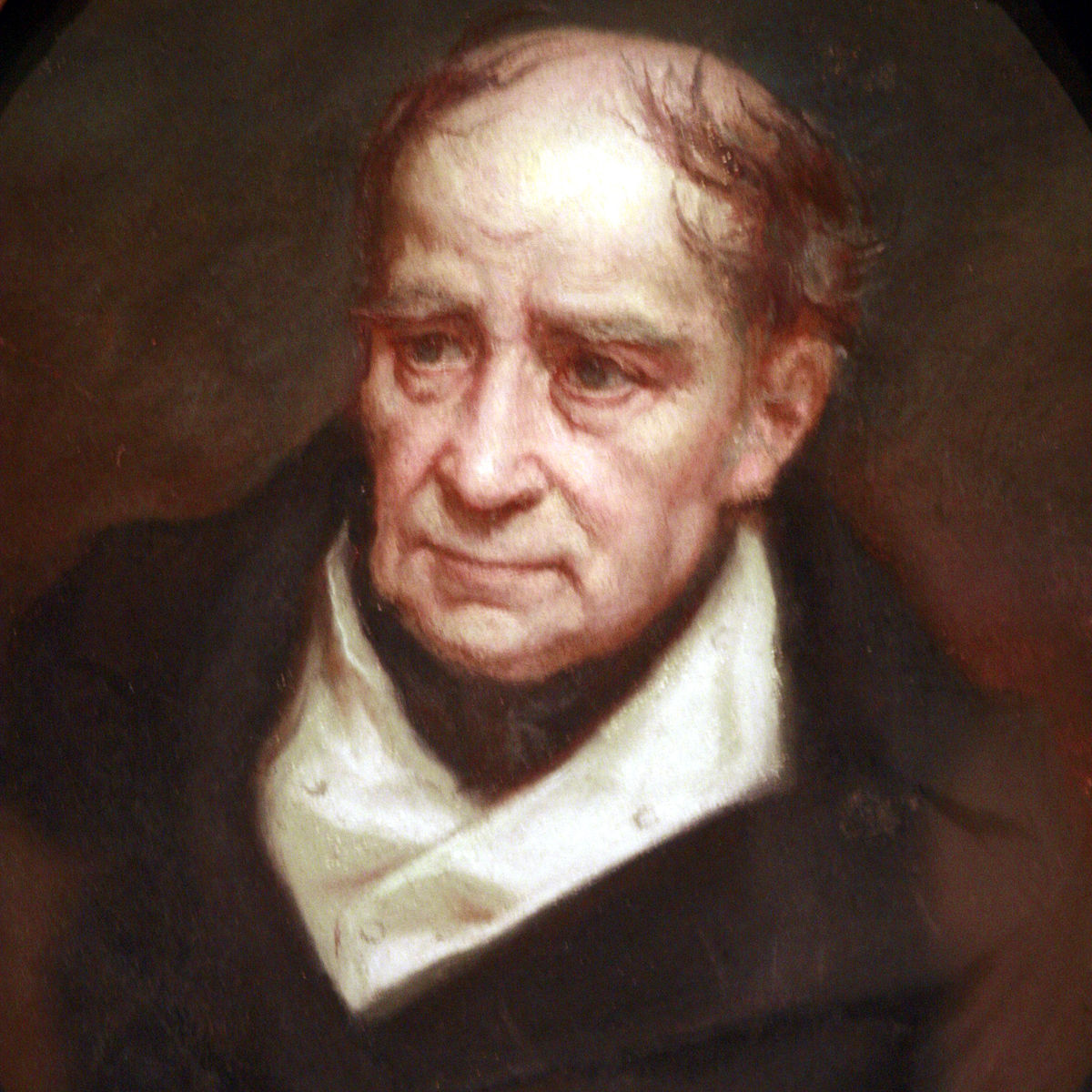
Jozéf Maria Hoëné Wronski was named Josef Hoëné after his birth in the town of Wolsztyn about 60 km south west of Poznań. His parents, from Czech families that had settled in western Poland, were Elzbieta Pernicka and Antoni Hoehne who was the municipal architect of Poznań. Josef Hoëné was educated in Poznań and Warsaw but in 1794 he became involved in the Kosciuszko Uprising.

Despite battles for independence, Russia and Prussia partitioned Poland in 1793. General Tadeusz Kosciuszko, a hero of the American War of Independence, returned to Poland in 1794 and gathered an army of Poles to again fight for independence. Hoëné joined Kosciuszko as second lieutenant in the artillery. After winning the battle of Raclawice and capturing Warsaw and Wilno, Kosciuszko's army was defeated by Russian and Prussian forces after a siege of Warsaw. Kosciuszko was wounded and taken prisoner by the Russian army. Hoëné Wronski was also taken prisoner, and made to serve in the Russian army which he did until 1797 when he was released having reached the rank of lieutenant colonel.

He spent the next years in Germany studying philosophy at a number of different universities. He enlisted in the Polish Legion at Marseilles, in France, and become a French citizen in 1800. Then in 1810 he moved to Paris and, in the same year, he married Victoire Henriette Sarrazin de Mountferrier, whose brother was the mathematician Alexandre Mountferrier. It was at this time that he adopted the surname Wronski but he did not use it consistently, rather alternately used Wronski and Hoehne.

His main work involved applying philosophy to mathematics, the philosophy taking precedence over rigorous mathematical proofs. He wrote on the philosophy of mathematics. His book Introduction to a course in mathematics was published in London in 1821. He criticised Lagrange's use of infinite series and introduced his own ideas for series expansions of a function. He introduced his Wronski series, whose coefficients are determinants now known as Wronskians. The term "Wronskian" was coined by the Scottish mathematician Thomas Muir (1844--1934) in 1882. However, Wronskian is a particular case of more general determinant known as Lagutinski determinant.

Let \( \left\{ f_1 , \ f_2 , \ \ldots , \ f_m \right\} \) be m functions that together eith threir first m-1 derivatives are continuous on an interval |a,b|. The Wronskian or the Wronskian determinant of \( \left\{ f_1 , \ f_2 , \ \ldots , \ f_m \right\} \) evaluated at \( x \in |a, b| \) is denoted by \( W[f_1, f_2 , \ldots , f_m ](x) \) or \( W(f_1, f_2 , \ldots , f_m ; x ) \) or simply \( W(x) \) and is defined to be the determinant

Each of the functions appearing in this determinant is to be evaluated at \( x \in |a, b| .\) ■

For the special case m = 2, the Wronskian takes the form

Lemma: For arbitrary functions \( \left\{ f , \ g_1 , \ \ldots , \ g_{n-1} \right\} , \) the Wronskian determinants satisfy the equation

In particular,

Theorem: Let \( \left\{ f_1 , \ f_2 , \ \ldots , \ f_{m} \right\} \) be m functions that together with their first m-1 derivatives are continuous on an open interval (a,b). If their Wronskian \( W \left[ f_1 , f_2 , \ldots , f_{m} \right] (x_0 ) \) is not equal to zero at some point \( x_0 \in (a,b) , \) then these functions \( f_1 , \ f_2 , \ \ldots , \ f_{m} \) are linearly independent on (a,b). Alternatively, if \( \left\{ f_1 , \ f_2 , \ \ldots , \ f_{m} \right\} \) are linearly dependent and they have m-1 first derivatives on the open interval (a,b), then their Wronskian \( W \left[ f_1 , f_2 , \ldots , f_{m} \right] (x ) \equiv 0\) for every x in (a,b).

Theorem: A finite set of linearly independent holomorphic (represented by convergent power series) functions has a nonzero Wronskian.

Theorem: Let \( \left\{ y_1 , \ y_2 , \ \ldots , \ y_{n} \right\} \) be the solutions of the n-th order linear differential equation

with continuous coefficients \( a_0 (x), \ a_1 (x) , \ \ldots , \ a_{n-1} (x) , \) defined on an open interval (a,b). Then functions \( \left\{ y_1 , \ y_2 , \ \ldots , \ y_{n} \right\} \) are linearly independent on this interval (a,b) if and only if their Wronskian never vanishes on (a,b). Alternatively, these functions \( \left\{ y_1 , \ y_2 , \ \ldots , \ y_{n} \right\} \) are linearly dependent on thids interval (a,b) if and only if \( W \left[ y_1 , y_2 , \ldots , y_{n} \right] (x ) \equiv 0\) is zero for all \( x \in (a,b). \)

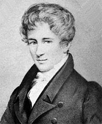
Theorem (Abel): If y₁ and y₂ are solutions of the second order linear differential equation

where p(x) and q(x) are continuous on an open interval (a,b), then the Wronskian \( W(x) = W[ y_1 , y_2 ] (x) \) is given by Here x₀ is any point from the interval (a,b). ■

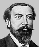
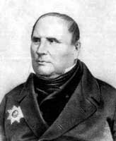
The above formula was derived by the greatest Norwegian mathematician Niels Henrik Abel (1802--1829) in 1827 for second order differential equation. In general case, namely, for the equation \( y^{(n)} + a_{n-1} (x)\, y^{(n-1)} + \cdots + a_1 (x)\, y' + a_0 (x)\, y =0 , \) the French mathematician Joseph Liouville (1809--18882) and the Russian mathematician Michel Ostrogradski (1801--1861) independently showed in 1838 that

Corallary: If the Wronskian W(x) of solutions \( y^{(n)} + a_{n-1} (x)\, y^{(n-1)} + \cdots + a_1 (x)\, y' + a_0 (x)\, y =0 , \) is zero at one point x₀ of an interval (a,b) where coefficients are continuous, then W(x) is 0 for all \( x \in (a,b) . \)

Corallary: If the Wronskian W(x) of solutions \( y^{(n)} + a_{n-1} (x)\, y^{(n-1)} + \cdots + a_1 (x)\, y' + a_0 (x)\, y =0 , \) is not zero, then it is not zero at ecery point of an interval where coefficients are continuous.

Theorem: There exists a fundamental set of solutions for the homogeneous linear n-th order linear differential equation in an interval where all coefficients are continuous.

Theorem: Consider the initial value problem

where p(x) and q(x) are continuous on an open interval (a,b) that contains the point x₀. Suppose that y₁ and y₂ are two linearly independent solutions of the homogeneous equation \( y'' + p(x)\, y' + q(x)\, y =0 . \) Then it is always possible to choose the constants C₁ and C₂ so that is the unique solution to the given initial value problem.

Theorem: Consider the linear differential equation

whose coefficients p and q are continuous on some open interval (a,b). Choose some point x₀ in it. Let y₁ be the solution of the above homogeneous linear equation that also satisfies the initial conditions and let y₂ be the solution of the above homogeneous linear equation that also satisfies the initial conditions Then y₁ and y₂ form a fundamental set of solutions to the equation \( y'' + p(x)\, y' + q(x)\, y =0 . \) ■

To check linearly independence of two functions, we have two options. First, two functions are linearly independent if and only if one of them is a constant multiple of another. Another option is to calculate the Wronskian if you know that these two functions are solutions of the same differential equation.

Example: verification of linearly dependence Example: calculating Wronskians

 

 

Return to Mathematica page

Return to the main page (APMA0330)
Return to the Part 1 (Plotting)
Return to the Part 2 (First Order ODEs)
Return to the Part 3 (Numerical Methods)
Return to the Part 4 (Second and Higher Order ODEs)
Return to the Part 5 (Series and Recurrences)
Return to the Part 6 (Laplace Transform) )
Return to the Part 7 (Boundary Value Problems)