This is a
tutorial made solely for the purpose of education and it was designed
for students taking Applied Math 0330. It is primarily for students who
have very little experience or have never used
Mathematica before and would like to learn more of the basics for this computer algebra system. As a friendly reminder, don't forget to clear variables in use and/or the kernel.
Finally, the commands in this tutorial are all written in bold black font,
while Mathematica output is in normal font. This means that you can
copy and paste all commands into Mathematica, change the parameters and
run them. You, as the user, are free to use the scripts for your needs to learn the Mathematica program, and have
the right to distribute this tutorial and refer to this tutorial as long as
this tutorial is accredited appropriately.
Return to computing page for the first course APMA0330
Return to computing page for the second course APMA0340
Return to Mathematica tutorial for the second course APMA0330
Return to Mathematica tutorial for the first course APMA0340
Return to the main page for the course APMA0340
Return to the main page for the course APMA0330
Return to Part III of the course APMA0330
Iteration is a fundamental principle in computer science. As the name suggests, it is a process that is repeated until
an answer is achieved or stopped. In this section, we study the process of iteration using repeated substitution.
More specifically, given a function g defined on the real numbers with real values and given a point x0 in the domain of g, the fixed point iteration is
which gives rise to the sequence \( \left\{ x_i \right\}_{i\ge 0} . \) If this sequence
converges to a point x, then one can prove that the obtained x is a fixed point of g, namely,
\[
x = g(x ) .
\]
When one wants to apply a function until the result stops changing,
Mathematica provides dedicated commands FixedPoint and FixedPointList
to achieve that. We present an alternative
approaches. One can also use NSolve command, as the following example shows.
Example: Suppose we want to find all the fixed points of
\( f(x)=x\, \sin (1/x) . \) Since it has infinitely many fixed points, so there would
in theory have infinitely many outputs.
Let f(x) be the following piecewise function:
f[x_] := Piecewise[{{x Sin [1/x], -1 <= x < 0 || 0 < x <= 1}}, 0]
Example: Suppose we need to solve the polynomial equation \( x^3 + 4\,x^2 -10 =0 , \) which we
rewrite as \( 4\, x^2 = 10 - x^3 . \) Taking square root, we reduce our problem to fixed point problem:
\( x = \frac{1}{2}\, \sqrt{10 - x^3} . \) Then we force Mathematica to use a given precision is to use Block
and make $MinPrecision equal to $MaxPrecision. So you can obtain your result as:
Mathematical operations on numbers of a given precision cannot guarantee the output to maintain the precision of the input numbers. In general precision will
decrease. The amount of decrease depends on the operations and some operations will cause precision to decrease significantly. If you want a specific precision
on the final result then the working precision should be higher than the desired output precision. Frequently, the working precision is done at twice the
desired output precision to allow for significant lose of precision during complex calculations. Sometimes using machine precision numbers will perform well.
Example:
Consider \( g(x) = 10/ (x^3 -1) \) and the fixed point iterative scheme \( x_{i+1} = 10/ (x^3_i -1) ,\) with the initial guess x0 = 2.
If you repeat the same procedure, you will be surprised that the iteration
is gone into an infinite loop without converging.
Theorem (Banach): Assume that the function g is continuous on the interval [a,b].
If the range of the mapping y = g(x) satisfies \( y \in [a,b] \) for all \( x \in [a,b] , \) then g has a fixed point in [a,b].
Furthermore, suppose that the derivative g'(x) is defined over (a,b) and that a positive constant (called Lipschitz constant) L < 1 exists with \( |g' (x) | \le L < 1 \) for all \( x \in (a,b) , \) then g has a unique fixed point P in [a,b]. ■
Stefan Banach (was born in 1892 in Kraków, Austria-Hungary and died 31 August
1945 in Lvov, Ukrainian SSR, Soviet Union) was a Polish mathematician who is
generally considered one of the world's most important and influential
20th-century mathematicians. He was one of the founders of modern functional
analysis, and an original member of the Lwów School of Mathematics. His major
work was the 1932 book, Théorie des opérations linéaires (Theory of Linear
Operations), the first monograph on the general theory of functional
analysis.
Rudolf Otto Sigismund Lipschitz (1832--1903) was a German mathematician who
made contributions to mathematical analysis (where he gave his name to the
Lipschitz continuity condition) and differential geometry, as well as number
theory, algebras with involution and classical mechanics.
Theorem: Assume
that the function g and its derivative are continuous on the interval
[a,b]. Suppose that \( g(x) \in [a,b] \) for all
\( x \in [a,b] , \) and the initial approximation
x0 also belongs to the interval [a,b].
If \( |g' (x) | \le K < 1 \) for all
\( x \in (a,b) , \) then the iteration
\( x_{i+1} = g(x_i ) \) will converge to the unique
fixed point \( P \in [a,b] . \) In this case,
P is said to be an attractive fixed point:
\( P= g(P) . \)
If \( |g' (x) | > 1 \) for all
\( x \in (a,b) , \) then the iteration
\( x_{i+1} = g(x_i ) \) will not converge to
P. In this case, P is said to be a repelling fixed point and
the iteration exhibits local divergence. ■
In practice, it is often difficult to check the condition
\( g([a,b]) \subset [a,b] \) given in the previous
theorem. We now present a variant of it.
Theorem: Let P be a fixed point of g(x), that is, \( P= g(P) . \) Suppose g(x) is differentiable on \( \left[ P- \varepsilon , P+\varepsilon \right] \quad\mbox{for some} \quad \varepsilon > 0 \) and g(x) satisfies the condition \( |g' (x) | \le K < 1 \) for all \( x \in \left[ P - \varepsilon , P+\varepsilon \right] . \) Then the sequence \( x_{i+1} = g(x_i ) , \) with starting point \( x_0 \in \left[ P- \varepsilon , P+\varepsilon \right] , \) converges to P.
Remark: If g is invertible then P is a fixed point of g if and only if P is a fixed point of g-1.
Remark: The above theorems provide only sufficient conditions. It is possible for a function to violate one or more of the
hypotheses, yet still have a (possibly unique) fixed point. ■
The Banach theorem allows one to find the necessary number of iterations for a given error "epsilon." It can be calculated by the following formula (a-priori error estimate)
Example: The function \( g(x) = 2x\left( 1-x \right) \) violates the hypothesis of the theorem because it is continuous everywhere \( (-\infty , \infty ) . \) Indeed, g(x) clearly does not map the interval \( [0.5, \infty ) \) into itself; moreover, its derivative \( |g' (x)| \to + \infty \) for large x. However, g(x) has fixed points at x = 0 and x = 1/2.
Example: Consider the equation
\[
x = 1 + 0.4\, \sin x , \qquad \mbox{with} \quad g(x) = 1 + 0.4\, \sin x .
\]
Note that g(x) is a continuous functions everywhere and \( 0.6 \le g(x) \le 1.4 \) for any \( x \in \mathbb{R} . \) Its derivative \( \left\vert g' (x) \right\vert = \left\vert 0.4\,\cos x \right\vert \le 0.4 < 1 . \) Therefore, we can apply the theorem and conclude that the fixed point iteration
we do not expect convergence of the fixed point iteration
\( x_{k+1} = 1 + 2\, \sin x_k . \)
II. Aitken's Algorithm
Alexander Aitken.
Sometimes we can accelerate or improve the convergence of an algorithm with
very little additional effort, simply by using the output of the algorithm to
estimate some of the uncomputable quantities. One such acceleration was
proposed by A. Aiken. Alexander Craig "Alec" Aitken was born in 1895 in
Dunedin, Otago, New Zealand and died in 1967 in Edinburgh, England, where he
spent the rest of his life since 1925. Aitken had an incredible memory
(he knew π to 2000 places) and could instantly multiply, divide and take
roots of large numbers. He played the violin and composed music to a very
high standard.
Suppose that we have an iterative process that generates a sequence of numbers \( \{ x_n \}_{n\ge 0} \)
that converges to α. We generate a new sequence \( \{ q_n \}_{n\ge 0} \) according to
where \( \Delta x_n = x_{n+1} - x_n \) is the forward finite difference.
Theorem (Aitken's Acceleration): Assume that the sequence \( \{ p_n \}_{n\ge 0} \) converges linearly to the limit p and that \( p_n \ne p \) for all \( n \ge 0. \) If there exists a real number A < 1 such that
converges to p faster than \( \{ p_n \}_{n\ge 0} \) in the sense that \( \lim_{n \to \infty} \, \left\vert \frac{p - q_n}{p- p_n} \right\vert =0 . \) ■
This algorithm was proposed by one of New Zealand's greatest mathematicians Alexander Craig "Alec" Aitken (1895--1967).
When it is applied to determine a fixed point in the equation \( x=g(x) , \) it consists in the following stages:
calculate x6 as the extrapolate of \( \left\{ x_3 , x_4 , x_5 \right\} . \) Continue this procedure, ad infinatum. ■
We assume that g is continuously differentiable, so according to Mean Value Theorem there exists
ξn-1 between α (which is the root of \( \alpha = g(\alpha ) \) ) and
xn-1 such that
Since we are assuming that \( x_n \,\to\, \alpha , \) we also know that
\( g' (\xi_n ) \, \to \,g' (\alpha ) ; \) thus, we can denote
\( \gamma_n \approx g' (\xi_{n-1} ) \approx g' (\alpha ) . \) Using this notation, we get
Now we present version 1 of Aitken extrapolation that does not take as much
advantage of acceleration as is possible.
Aitken Extrapolation, Version 1

x1 = g(x0)

x2 = g(x1)

for k=1 to n do

	if (dabs[x1 - x0) > 1.d-20) then

		gamma = (x2 - x1)/(x1 - x0)

	else

		gamma = 0.0d0

	endif

	q = x2 + gamma*(x2 - x1)/(1 - gamma)

	if(abs(q - x2) < error) then

		alpha = q

		stop

	endif

	x = g(x2)

	x0 = x1

	x1 = x2

	x2 = x

enddo
Since division by zero---or a very small number---is possible in the algorithm's computation of γ, we put in a
conditional test: Only if the denominator is greater than 10-20 do we carry through the division.
Example: Repeat the previous example according to version 1.
III. Steffensen's Acceleration
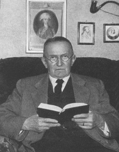
Johan Steffensen.
Johan Frederik Steffensen (1873--1961) was a Danish mathematician, statistician, and actuary who did research in the fields of calculus of finite differences and interpolation. He was professor of actuarial science at the University of Copenhagen from 1923 to 1943. Steffensen's inequality and Steffensen's iterative numerical method are named after him.
When Aitken's process is combined with the fixed point iteration in Newton's method, the result is called Steffensen's acceleration. Starting with p0, two steps of Newton's method are used to compute \( p_1 = p_0 - \frac{f(p_0 )}{f' (p_0 )} \) and \( p_2 = p_1 - \frac{f(p_1 )}{f' (p_1 )} , \) then Aitken's process is used to compute \( q_0 = p_0 - \frac{\left( \Delta p_0 \right)^2}{\Delta^2 p_0} . \) To continue the iteration set \( q_0 = p_0 \) and repeat the previous steps. This means that we have a fixed-point iteration:
If at some point \( \Delta^2 p_n =0 \) (which appears in the denominator), then we stop and select the current value of pn+2 as our approximate answer.
Steffensen's acceleration is used to quickly find a solution of the fixed-point equation x = g(x) given an initial approximation p0. It is assumed that both g(x) and its derivative are continuous, \( | g' (x) | < 1, \) and that ordinary fixed-point iteration converges slowly (linearly) to p.
Now we present the pseudocode of the algorithm that provides faster convergence. Note that we check again for division by small numbers before computing
γ.
Steffensen's acceleration

for k=1 to n do

	x1 = g(x0)

	x2 = g(x1)

	if (dabs[x1 - x0) > 1.d-20) then

		gamma = (x2 - x1)/(x1 - x0)

	else

		gamma = 0.0d0

	endif

	x0 = x2 + gamma*(x2 - x1)/(1 - gamma)

	if(abs(x0 - x2) < error) then

		alpha = x0

		stop

	endif

enddo
Example: Repeat the previous example according
to version 2.
V. Wegstein's Method
To solve the fixed point problem \( g(x) =x , \) the following algorithm, presented in
J.H. Wegstein, Accelerating convergence of iterative processes, Communications of the Association for the Computing Machinery (ACM), 1, 9--13, 1958. can be used
for \( n=0,1,2,\ldots . \) Wegstein (1958) found
that the iteration converge differently
depending on the value of q.
q < 0
Convergence is monotone
0 < q < 0.5
Convergence is oscillatory
0.5 < q < 1
Convergence
q > 1
Divergence
Wegstein's method depends on two first guesses x0 and x1 and poor start may cause the process to fail, converge to another root, or, at best, add unnecessary number of iterations.
Example: Repeat the previous example according to Wegstein's method.
Return to the main page (APMA0330)
Return to the Part 1 (Plotting)
Return to the Part 2 (First Order ODEs)
Return to the Part 3 (Numerical Methods)
Return to the Part 4 (Second and Higher Order ODEs)
Return to the Part 5 (Series and Recurrences)
Return to the Part 6 (Laplace Transform)
Return to the Part 7 (Boundary Value Problems)