Preface

This is a tutorial made solely for the purpose of education and it was designed for students taking Applied Math 0330. It is primarily for students who have very little experience or have never used Mathematica before and would like to learn more of the basics for this computer algebra system. As a friendly reminder, don't forget to clear variables in use and/or the kernel.

Finally, the commands in this tutorial are all written in bold black font, while Mathematica output is in normal font. This means that you can copy and paste all commands into Mathematica, change the parameters and run them. You, as the user, are free to use the scripts for your needs to learn the Mathematica program, and have the right to distribute this tutorial and refer to this tutorial as long as this tutorial is accredited appropriately.

Plotting Solutions of ODEs

When Mathematica is capable to find a solution (in explicit or implicit form) to an initial value problem, it can be plotted as follows. Let us consider the initial value problem

In this command sequence, I am first defining the differential equation that I want to solve. In this line, I define the equation and the initial condition as well as the independent and dependent variables.
In the second line, I am commanding Mathematica to evaluate the given differential equation and plot its result. I then command Mathematica to solve the equation and plot the given result of the initial value problem for the range listed above. Typing these two commands together allows Mathematica to solve the initial value problem for you and to graph the initial value problem's solution.

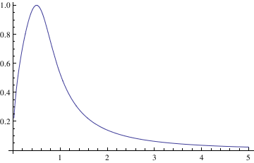
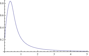
If you need to plot a sequence of solutions with different initial conditions, one can use the following script:

DSolve::bvnul: For some branches of the general solution, the given
boundary conditions lead to an empty solution. >>

DSolve::bvnul: For some branches of the general solution, the given
boundary conditions lead to an empty solution. >>