This tutorial contains many Mathematica scripts. You, as the user, are free to use all codes for your needs, and have the right to distribute this tutorial and refer to this tutorial as long as this tutorial is accredited appropriately. Any comments and/or contributions for this tutorial are welcome; you can send your remarks to <Vladimir_Dobrushkin@brown.edu>
Return to computing page for the second course APMA0330
Return to Mathematica tutorial page for the first course
Return to Mathematica tutorial page for the second course
Return to the main page for the course APMA0330
Return to the main page for the course APMA0340
3.0.0. Introduction
Ordinary differential equations are at the heart of our perception of the physical universe. For this reason numerical methods for their solutions is one of the oldest and most successful areas of numerical computations.
It would be very nice if discrete models provide calculated solutions to differential (ordinary and partial) equations exactly, but of course they do not. In fact in general they could not, even in principle, since the solution depends on an infinite amount of initial data. Instead, the best we can hope for is that the errors introduced by discretization will be small when those initial data are resonably well-behaved.
In this chapter, we discuss some simple numerical method applicable to first order ordinary differential equations in normal form subject to the prescribed initial condition:
The finite diference approximations have a more complecated "physics" than the equations they are designed to simulate. In general, finite recurrences usually have more propertities than their continuous anologous counterparts. However, this arony is no paradox; the finite differences are used not because the numbers they generate have simple properties, but because those numbers are simple to compute.
Numerical methods for the solution of ordinary differential equations may be put in two categories---numerical integration (e.g., predictor-corrector) methods and Runge--Kutta methods. The advantages of the latter are that they are self-starting and easy to program for digital computers but neither of these reasons is very compelling when library subroutines can be written to handle systems of ordinary differential equations. Thus, the greater accuracy and the error-estimating ability of predictor-corrector methods make them desirable for systems of any complexity. However, when predictor-corrector methods are used, Runge--Kutta methods still find application in starting the computation and in changing the interval of integration.
In this chapter, we discuss only discretization methods that have the common feature that they do not attempt to approximate the actual solution y = φ (x) over a continuous range of the independent variable. Instead, approximate values are sought only on a set of discrete points \( x_0 , x_1 , x_2 , \ldots . \) This set is usually called grid or mesh. For simplicity, we assume that that these mesh points are equidistance: \( x_n = a+ n\,h , \quad n=0,1,2,\ldots . \) The quantity h is then called the stepsize, stepwidth, or simply the step of the method. Generally speaking, a discrete variable method for solving a differential equation consists in an algorithm which, corresponding to each lattice point xn, furnishes a number yn which is to be regarded as an approximation to the true value \( \varphi (x_n ) \) of the actual solution at the point xn.
3.0.1. Errors in Numerical Approximations
The main question of any approximation is whether the numerical approximations \( y_1 , y_2 , y_3 , \ldots \) approach the corresponding values of the actual solution? We want to use a step size that is small enough to ensure the required accuracy. An unnecessarily small step length slows down the calculations and in some cases may even cause a loss of accuracy.
There are three fundamental sources of error in approximating the solution of an initial value problem numerically.
- The formula, or algorithm, used in the calculations is an approximating one.
- Except for the first step, the input data used in the calculations are only approximations to the actual values of the solution at the specified points.
- The computer used for the calculations has finite precision; in other words, at each stage only a finite number of digits can be retained.
Let us temporarily assume that our computer can execute all computations exactly; that is, it can retain infinitely many digits (if necessary) at each step. Then the difference En between the actual solution \( y = \phi (x) \) of the initial value problem \( y' = f(x,y), \quad y(x_0 ) = y_0 \) and its numerical approximation yn at the point x = xn is given by
However, in reality we must carry out the calculations using finite precision arithmetic because of the limited accuracy of any computing equipment. This means that we can keep only a finite number of digits at each step. This leads to a round-off error Rn defined by
Therefore, the total error is bounded by the sum of the absolute values of the global truncation and round-off errors. The round-off error is very difficult to analyze and it is beyond of the scope of our topic. To estimate the global error, we need one more definition.
As we carry the solution over many steps we would expect the values yn and \( \phi (x_n ) \) to diverge further and further apart. The local truncation error is concerned only with the direvgence produced within the present step so that it is appropriate to reinitialize yn to the value of \( \phi (x_{n} ) \) in studying this source of error. The corresponding solution to the initial value problem
3.0.2. Fundamental Inequality
We start with estimating elements of sequences.
Theorem: Suppose that elements of a sequence \( \left\{ \xi_n \right\} , \ n=0,1,2,\ldots , \) satisfy the inequalities of the form
Theorem: If A is a quantity of the form 1 + δ , then \( A = 1 + \delta < e^{\delta} \) and we have
Recall that a function f is said to satisfy Lipschitz's condition (or being Lipschitz continuous) on some interval if there exists a positive constant L such that
for every pair of points y1 and y2 from the given interval.■
Rudolf Otto Sigismund Lipschitz (1832--1903) was born in Königsberg, Germany (now Kaliningrad, Russia). He entered the University of Königsberg at the age of 15 and completed his studies at the University of Berlin, from which he was awarded a doctorate in 1853. By 1864 he was a full professor at the University of Bonn, where he remained the rest of his professional life.Theorem (Fundamental Inequality): Let f(x,y) be a continuous function in the rectangle \( [a,b] \times [c,d] \) and satisfying the Lipschitz condition
3.0.3. Numerical Solution using DSolve and NDSolve
A complete analysis of a differential equation is almost impossible without utilizing computers and corresponding graphical presentations. We are not going to pursue a complete analysis of numerical methods, which usually requires:
- an understanding of computational tools;
- an understanding of the problem to be solved;
- construction of an algorithm which will solve the given mathematical problem.
In this chapter, we concentrate our attention on presenting some simple numerical algorithms for finding solutions of the initial value problems for the first order differential equations in the normal form:
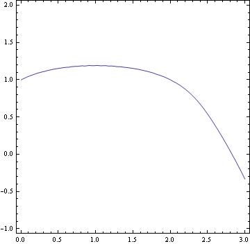
A general approach for determing numerically solutions of the initial value problems and then plot them using Mathematica's capability is as follows. We demostrate all steps on the following initial value problem (IVP, for short):
Plot[y[x] /. a, {x,0,3}]
To see a numerical value at, say x=3.0, we type:
ContourPlot[psi[x, y] == 0, {x, 0, 2}, {y, -1, 3}, ContourLabels->True, ColorFunction->Hue]

http://library.wolfram.com/infocenter/Books/8503/AdvancedNumericalDifferentialEquationSolvingInMathematicaPart1.pdf
IV. Regular Plotting vs Log-Plotting
Plotting the absolute value of the errors for Taylor approximations, such as the ones from the previous example, is fairly easy to do in normal plotting.
The normal plotting procedure involves taking all of the information regarding the Taylor approximations and putting them into one file, then calculate the exact solution, then find the difference between each approximation and the exact solution, and plotting the solution.
Looking at the code, the syntax is pretty much self-explanatory. The only part that may confuse students is the syntax for the plot command. The plot command need not be in the same syntax as the file has it. If you wish to, you can alter the syntax to form a curve instead of dots.
Log-plotting is not much different than plotting normally. In other programs such as Mathematica, there are a couple of fixes to make, but in Maple only one line of code is required, as seen in the file. Make sure that before you use the logplot command to open the plots package.
Now, let’s compare the exact value and the values determined by the polynomial approximations and the Runge-Kutta method.
| x values | Exact | First Order Polynomial | Second Order Polynomial | Third Order Polynomial | Runge-Kutta Method |
| 0.1 | 1.049370088 | 1.050000000 | 1.049375000 | 1.049369792 | 1.049370096 |
| 0.2 | 1.097463112 | 1.098780488 | 1.097472078 | 1.097462488 | 1.097463129 |
| 0.3 | 1.144258727 | 1.146316720 | 1.144270767 | 1.144257750 | 1.144258752 |
| 0.4 | 1.189743990 | 1.192590526 | 1.189758039 | 1.189742647 | 1.189744023 |
| 0.5 | 1.233913263 | 1.237590400 | 1.233928208 | 1.233911548 | 1.233913304 |
| 0.6 | 1.276767932 | 1.281311430 | 1.276782652 | 1.276765849 | 1.276767980 |
| 0.7 | 1.318315972 | 1.323755068 | 1.318329371 | 1.318313532 | 1.318316028 |
| 0.8 | 1.358571394 | 1.364928769 | 1.358582430 | 1.358568614 | 1.358571457 |
| 0.9 | 1.397553600 | 1.404845524 | 1.397561307 | 1.397550500 | 1.397553670 |
| 1.0 | 1.435286691 | 1.443523310 | 1.435290196 | 1.435283295 | 1.435286767 |
| Accuracy | N/A | 99.4261% | 99.99975% | 99.99976% | 99.99999% |
You will notice that compared to the Euler methods, these methods of approximation are much more accurate because they contains much more iterations of calculations than the Euler methods, which increases the accuracy of the resulting y-value for each of the above methods.
Horner's rule
The most efficient way to evaluate a polynomial is by nested multiplication. If we have a polynomial of degree n
Horner's rule for polynomial evaluation

% the polynomial coefficients are stored in the array a(j), j=0,1,..,n

% px = value of polynomial upon completion of the code


px = a(n)

for k = n-1 downto 0

	px = a(k) + px*x

endfor
Similar algorithm for evaluating derivative of a polynomial:
Horner's rule for polynomial derivative evaluation

% the polynomial coefficients are stored in the array a(j), j=0,1,..,n

% dp = value of derivative upon completion of the code


dp = n*a(n)

for k = n-1 downto 1

	dp = k*a(k) + dp*x

endfor
William George Horner (1786--1837) was born in Bristol, England, and spent much of his life as a schoolmaster in
Bristol and, after 1809, in Bath. His paper on solving algebraic equations, which contains the algorithm we know as
Horner's rule, was published in 1819, although the Itarian mathematician Ruffini had previously
published a very similar idea.
here is a more efficient algorithm for polynomial evaluation:
A more efficient implementation of Horner's rule for polynomial evaluation

% the polynomial coefficients are stored in the array a(j), j=0,1,..,n

% b(n) = value of polynomial upon completion of the code


b(0) = a(n)

for k = 1 to n

	b(k) = x*b(k-1) + a(n-k)

endfor


% c(n-1) = value of derivative upon completion of the code


c(0) = b(0)

for k = 1 to n-1

	c(k) = x*c(k-1) + b(k)

endfor
3.0.4. Applications
Example:
A 500 liter container initially contains 10 kg of salt. A brine mixture of 100 gramms
of salt per liter is entering the container at 6 liter per minute. The well-mixed contents
are being discharged from the tank at the rate of 6 liters per minute. Express the amount
of salt in the container as a function of time.
Salt is coming at the rate: 6*(0.1)=0.6 kg/min
d yin /dt =0.6 ; d yout/dt = 6x/500
dx/dt = 0.6 -6x/500 ; x(0)=10
Suppose that the rate of discharge is reduced to 5 liters per minute.
SolRule[t_] = Apart[x[t] /. First[%]]
10 (500 + t)^5))(3125000000000000 + 187500000000000 t +
937500000000 t^2 + 2500000000 t^3 + 3750000 t^4 + 3000 t^5 +
t^6)}}
Out[2]= 50 + t/10 - 1250000000000000/(500 + t)^5
To check the answer:
Together[SolRule'[t] == Together[6/10 - 5*SolRule[t]/(500 + t)]]
SolRule[0]
Out[4]= True
Out[5]= 10