Preface
This tutorial was made solely for the purpose of education and it was designed for students taking Applied Math 0330. It is primarily for students who have very little experience or have never used Mathematica before and would like to learn more of the basics for this computer algebra system. As a friendly reminder, don't forget to clear variables in use and/or the kernel.
Finally, the commands in this tutorial are all written in bold black font, while Mathematica output is in normal font. This means that you can copy and paste all commands into Mathematica, change the parameters and run them. You, as the user, are free to use the scripts for your needs to learn the Mathematica program, and have the right to distribute this tutorial and refer to this tutorial as long as this tutorial is accredited appropriately.
Return to computing page for the second course APMA0340
Return to Mathematica tutorial for the second course APMA0340
Return to Mathematica tutorial for the first course APMA0330
Return to the main page for the course APMA0340
Return to the main page for the course APMA0330
Return to Part IV of the course APMA0330
Pendulum
I. Pendulum Equation
The simple pendulum is of historic and basic importance. Its approximate isochronism, was first discovered by Galileo, who is said to check the constancy of the period of the small oscillations of a pendulum by comparing them with his heartbeat. In hands of Newton, pendulum provided the first evidence that inertial and gravitational masses are proportional. Until relatively recently, the plane pendulum yielded the most accurate and convenient method for measuring the local gravitational acceleration.
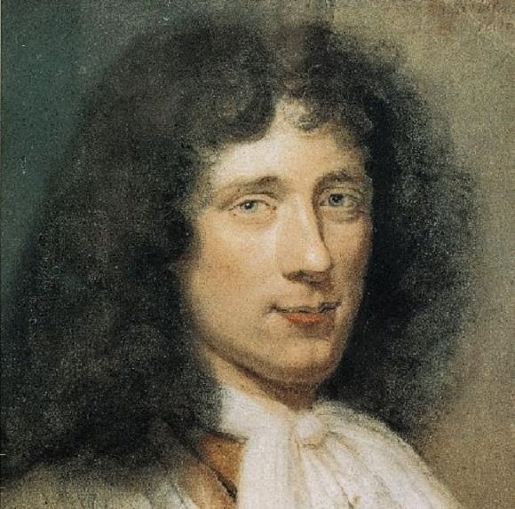
There is no doubt that the first person who investigated and established the mathematical theory and properties of the pendulum was a prominent Dutch mathematician and scientistt named Christiaan Huygens (this spelling of his name is taken from the title of his 1658 book Horologium Oscillatorium). The main point of Huygens' (1629--1695) discovery was that the curve in which a pendulum particle (or bob) hangs by a string of insensible weight must move in order to be isochronous in its vibrations, and is not a circle, but a cycloid.
The pendulum consists of a bob of mass m attached to the end of a light inextensible rod of length \( \ell \) with the motion taking place in a vertical plane. Such pendulum is usually referred to as a simple pendulum. Let θ be the angular coordinate of m measured counterclockwise from the down position. The kinetic and potential energies are
Simple pendulum equation \( \ddot{\theta} + \omega_0^2 \sin \theta =0 , \) although straightforward in appearance, is in fact rather difficult to solve because of the non-linearity of the term \( \sin \theta . \) In order to obtain the exact solution, this equation is multiplied by the integrating factor \( \dot{\theta} = {\text d}\theta / {\text d} t, \) so that it becomes
Module[{run, sol, z, app, a},
If[run == 10, run = 0];
sol = DSolve[{y''[x] + (9.8/l)*y[x] == 0, y[0] == int, y'[0] == 0}, y, x];
z[x_] := y[x] /. sol;
app = NDSolve[{\[Theta]1''[t] + (9.8/l)*Sin[\[Theta]1[t]] == 0, \[Theta]1[0] == int, \[Theta]1'[0] == 0}, \[Theta]1, {t, 0, 10}];
a[t_] := \[Theta]1[t] /. First[app];
Grid[{{
Graphics[{
{Thick, Line[{{0, 0}, {l*Sin[a[r]], -l*Cos[a[r]]}}]}, {Darker[Green], Disk[{0, 0}, .03]}, {Purple,
Disk[{l*Sin[a[r]], -l*Cos[a[r]]}, 0.1 Power[(30 m)/(4 \[Pi]), (3)^-1]]}},
PlotRange -> {{-3.4, 3.4}, {.5, -3.4}},
ImageSize -> {250, 250}],
Plot[{a[t], z[t]}, {t, 0, 10},
PlotRange -> {{0, 10}, {-1.6, 1.6}},
PlotStyle -> {{Thick, Blue}, {Red}}, ImageSize -> {250, 250},
AspectRatio -> 1.2, Frame -> True,
PlotLegends`PlotLegend -> {"numerical", "sin(\[Theta]) = \[Theta]"},
FrameLabel -> {"time", "displacement"},
Epilog -> {Blue, PointSize[.06], Point[{r, a[r]}]}]}}]],
{{int, \[Pi]/3., "initial angle \[Theta](0)"}, \[Pi]/16., \[Pi]/2., Appearance -> "Labeled"},
Delimiter,
{{m, 4, "mass m"}, 1, 10, .01, Appearance -> "Labeled"},
{{l, 2.25, "length L"}, 1, 3, .01,
Appearance -> "Labeled"}, {{r, 0, "release system"}, 0, 10, .01,
ControlType -> Trigger, AnimationRate -> .5},
TrackedSymbols :> {int, m, l, r},
Initialization :> Get["PlotLegends`"]]
II. Pendulum Equation with Resistance
The resistance of the air acts on both the pendulum ball and the pendulum wire. It causes the amplitude to decrease with time and increases the period of oscillation slightly. The drag force is proportional to the velocity for values of the Reynolds number of the order 1 or less. For values of the Reynolds number of order \( 10^3 \) to \( 10^5 , \) the force is proportional to the square of the velocity. The maximum Reynolds number based on diameter for the ball is 1100, where the quadratic force law should apply, while the maximum value based on the diameter of a wire is about 6, where the linear force law should prevail.
Since the damping force is neither linear nor quadratic, but rather a combination of the two, it makes sense to establish a damping function which contains both effects simultaneously. Therefore, the pendulum equation becomes
where the linear damping coefficient \( \alpha = \kappa /m , \) describes air resistance due to the wire, the quadratic damping coefficient β is due to air drag on the pendulum bob, and the third damping term \( \quad \epsilon = c\ell /(2m) \) is necessary for taking into count the bearing, which is subject to dry friction (Coulomb damping). Here \( \quad \omega_0 = \left( g/\ell \right)^{1/2} ,\) and \( \mbox{sign}(x) = \begin{cases} 1, & \ x>0, \\ -1, & \ x<0. \end{cases} \)
Analysis of the experimental data gives the following values of the parameters (Robert A. Nelson and M.G. Olsson, "The pendulum---rich physics from a simple system," American Journal of Physics, Vol. 54, No 2, 112--121, 1986):
This can be done by assigning constant values to α,
ε and ω when using the NDSolve command, getting three
different functions in respect to three different α values,
and using the Plot command to plot the three functions in one graph
NDSolve[{y''[x] == -10*2*y'[x] - Sin[y[x]], y[0] == 0.7, y'[0] == 0}, y[x], {x, 0, 1000}]
numsol2 =
NDSolve[{y''[x] == -1*2*y'[x] - Sin[y[x]], y[0] == 0.7, y'[0] == 0}, y[x], {x, 0, 1000}]
numsol3 =
NDSolve[{y''[x] == -0.1*2*y'[x] - Sin[y[x]], y[0] == 0.7, y'[0] == 0}, y[x], {x, 0, 1000}]
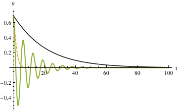
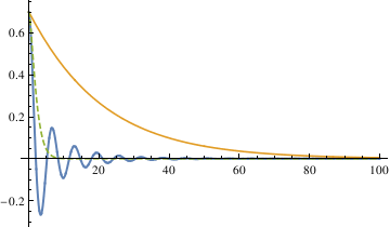
Plot[Evaluate[y[x] /. {numsol1, numsol2, numsol3}], {x, 0, 100}, PlotRange -> All, PlotStyle -> {GrayLevel[0.1], Dashed, Thick}, AxesLabel -> {"t", "\[Theta]"}, PlotLegends -> {"\[Alpha]=10", "\[Alpha]=1", "\[Alpha]=0.1"}]
Another method is to set up a function that takes θ0, ω0, α, ε and tmax as inputs and outputs for a function of θ
Module[{\[Theta]}, \[Theta] /. First[ NDSolve[{ \[Theta]''[t] == -Sin[\[Theta][t]] - 2 \[Alpha] \[Theta]'[ t] - \[Epsilon] Sign[\[Theta]'[t]] (\[Theta]'[t])^2, \[Theta][0] == \[Theta]0, \[Theta]'[0] == \[Omega]0}, \[Theta], {t, 0, tmax}
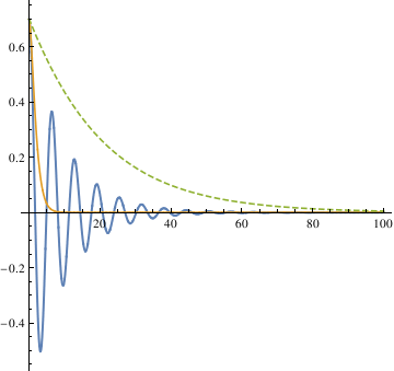
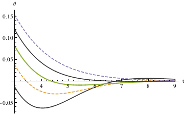
The three different methods all get the same result, from which we can see that the largest damping coefficient does not stop the pendulum the fastest. So the qualitative difference among the three different coefficients is that when α is 0.1, the pendulum oscillates (crosses 0). In other cases, the pendulum does not oscillate (does not cross 0).
The critical damping value is the damping coefficient that stops the pendulum the fastest.
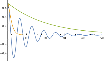
In order to find out the critical damping value of alpha, first we need to define the stop interval, because the pendulum will end up always being in very small oscillation.
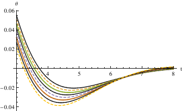
The first method defined - 0.035 < θ < 0.035 as the stop interval. By plotting different functions of θ with different alpha values (0.6, 0.7, 0.8, 0.9, 1.0) in one graph, you can see that α = 0.7 starts to be in the range [-0.035, 0.035] the fastest.
NDSolve[{y''[x] == -0.6*2*y'[x] - Sin[y[x]], y[0] == 0.7, y'[0] == 0}, y[x], {x, 0, 1000}]
numsolb1 =
NDSolve[{y''[x] == -0.7*2*y'[x] - Sin[y[x]], y[0] == 0.7, y'[0] == 0}, y[x], {x, 0, 1000}]
numsolc1 =
NDSolve[{y''[x] == -0.8*2*y'[x] - Sin[y[x]], y[0] == 0.7, y'[0] == 0}, y[x], {x, 0, 1000}]
numsold1 =
NDSolve[{y''[x] == -0.9*2*y'[x] - Sin[y[x]], y[0] == 0.7, y'[0] == 0}, y[x], {x, 0, 1000}]
numsolf1 =
NDSolve[{y''[x] == -1.0*2*y'[x] - Sin[y[x]], y[0] == 0.7, y'[0] == 0}, y[x], {x, 0, 1000}]
NDSolve[{y''[x] == -0.74*2*y'[x] - Sin[y[x]], y[0] == 0.7, y'[0] == 0}, y[x], {x, 0, 1000}]
numsolb =
NDSolve[{y''[x] == -0.73*2*y'[x] - Sin[y[x]], y[0] == 0.7, y'[0] == 0}, y[x], {x, 0, 1000}]
numsolc =
NDSolve[{y''[x] == -0.72*2*y'[x] - Sin[y[x]], y[0] == 0.7, y'[0] == 0}, y[x], {x, 0, 1000}]
numsold =
NDSolve[{y''[x] == -0.71*2*y'[x] - Sin[y[x]], y[0] == 0.7, y'[0] == 0}, y[x], {x, 0, 1000}]
numsolf =
NDSolve[{y''[x] == -0.70*2*y'[x] - Sin[y[x]], y[0] == 0.7, y'[0] == 0}, y[x], {x, 0, 1000}]
numsolg =
NDSolve[{y''[x] == -0.69*2*y'[x] - Sin[y[x]], y[0] == 0.7, y'[0] == 0}, y[x], {x, 0, 1000}]
numsolh =
NDSolve[{y''[x] == -0.68*2*y'[x] - Sin[y[x]], y[0] == 0.7, y'[0] == 0}, y[x], {x, 0, 1000}]
numsoli =
NDSolve[{y''[x] == -0.67*2*y'[x] - Sin[y[x]], y[0] == 0.7, y'[0] == 0}, y[x], {x, 0, 1000}]
When α = 0.85, the pendulum settles in the range faster than when α = 1. So the critical value may be smaller than 0.85. Try the mid value of 0.85 and 0.7. Finally, the answer yielded from this method is 0.81.
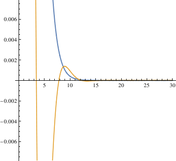
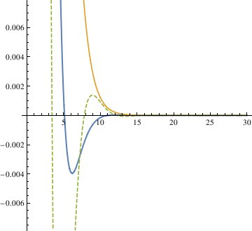
The third method defines the stop interval as not passing 0 in the time span 0 < t \ < 500, uses a function piano to check if the pendulum oscillates.
\[CapitalOmega]0 = 1;
listofsolutions = {};
listofvaluesfor\[Alpha] = Range[0, 2, .0005];
pendulumeq = \[Theta]''[t] + 2*\[Alpha]*\[Theta]'[t] + \[CurlyEpsilon]* Sign[\[Theta]'[t]]*((\[Theta]'[t])^2) + (\[CapitalOmega]0^2)* Sin[\[Theta][t]] == 0;
Catch[If[FindMinValue[ evaluatedlistofsolutions[[key]], {t, 0, 500}] > 0, Throw[key], Throw[906]]];
Module[{\[Theta]}, \[Theta] /. First[ NDSolve[{ \[Theta]''[t] == -Sin[\[Theta][t]] - 2 \[Alpha] \[Theta]'[ t] - \[Epsilon] Sign[\[Theta]'[t]] (\[Theta]'[t])^2, \[Theta][0] == \[Theta]0, \[Theta]'[0] == \[Omega]0}, \[Theta], {t, 0, tmax}] ]]
III. A Real Pendulum
A real pendulum bob has a finite size and the suspension wire has a mass. In addition, the wire connections to the bob and the support may have some structure. Normally, pendulum osccilations take place in air. All such effects should be taking into account in physical pendulum equation.
By Archimedes's principle, the apparent weight of the bob is reduced by the weight of the displaced air. This property has the effect of increasing the period since the effective gravity is decresing. The kinetic energy of the system is partly effected by the air by adding mass to the bob's inertia (but not weight) proportional to the mass of the displaced air. The need for the added mass correction was noted by Friedrich Bessel (1784--1846) in 1828. (It was discovered independently by Pierre Du Buat (1734--1809) in 1786, but only Bessel's work attracted attention to his result.) The dependence of added mass on viscosity was derived by George Stokes (1819--1903) in 1859.
The length of the pendulum is incresed by stretching of the wire due to the weight of the bob. The effective spring constant for a wire of rest length \( \ell_0 \) is
There is also dynamic stretching of teh wire from the apparent centrifugal and Coriolis forces acting on the bob during mortion. The corresponding mathematical model leads to a system of differential equations, which is a topic of the second course. See M.G. Olson, American Journal of Physics, Vol. 44, 1211, 1976.
IV. Driven Pendulum
A driven pendulum may exhibit a chaotic motion. It consists of a mass m fixed at a distance \( \ell \) from a pivot which is subject to a vertical oscillation \( y = A\, \cos \left( \omega \, t \right) . \) Let θ be the angular coordinate of m measured counterclockwise from the down position, and \( \phi = \pi - \theta \) the complementary displacement measured clockwise from the up orientation. The kinetic and potential energies are
V. Rocking Rigid Pendulum
minus = Polygon[{{1/2, 0}, {1/2, 1/4}, {4, 1/4}, {4, 0}}]
a = Show[Graphics[{Pink, minus}], Graphics[{Pink, plus}]]
line1 = Graphics[Line[{{-2, -3.5}, {0, 0.6}}], PlotRange -> {{-2, 2}, {-4, 1}}]
line2 = Graphics[Line[{{-0.85, 1.0}, {0.8, 0.25}}], PlotRange -> {{-2, 2}, {-4, 1}}]
makeArrowPlot[g_Graphics, ah_: 0.05, dx_: 1*^-6, dy_: 1*^-6] :=
Module[{pr = PlotRange /. Options[g, PlotRange], gg, lhs, rhs},
gg = g /. GraphicsComplex -> (Normal[GraphicsComplex[##]] &);
lhs := Or @@
Flatten[{Thread[Abs[#[[1, 1, 1]] - pr[[1]]] < dx], Thread[Abs[#[[1, 1, 2]] - pr[[2]]] < dy]}] &;
rhs := Or @@ Flatten[{Thread[Abs[#[[1, -1, 1]] - pr[[1]]] < dx], Thread[Abs[#[[1, -1, 2]] - pr[[2]]] < dy]}] &;
gg = gg /.
x_Line?(lhs[#] && rhs[#] &) :> {Arrowheads[{-ah, ah}], Arrow @@ x};
gg = gg /. x_Line?lhs :> {Arrowheads[{-ah, 0}], Arrow @@ x};
gg = gg /. x_Line?rhs :> {Arrowheads[{0, ah}], Arrow @@ x};
gg]
curve = Plot[{-Sqrt[9 - x^2]}, {x, -2.2, 2.2}, PlotStyle -> {Thick, Dashed}, Axes -> False] // makeArrowPlot
Show[a, line1, line2, curve]
minus = Polygon[{{1/2, 0}, {1/2, 1/4}, {4, 1/4}, {4, 0}}]
a = Show[Graphics[{Pink, minus}], Graphics[{Pink, plus}]]
line1 = Graphics[Line[{{-2, -3.5}, {0, 0.6}}], PlotRange -> {{-2, 2}, {-4, 1}}]
line2 = Graphics[Line[{{-0.85, 1.0}, {0.8, 0.25}}], PlotRange -> {{-2, 2}, {-4, 1}}]
p2 = Graphics[{Dashed, Arrow[{{-0.66, -0.8}, {-0.66, -3.8}}]}]
point = Graphics[{PointSize[Large], Green, Point[{-0.66, -0.8
t1 = Graphics[ Text[Style["\[Theta]", FontSize -> 14, Red], {-1.0, -2.4}]]
t2 = Graphics[Text[Style["G", FontSize -> 14, Blue], {-1.0, -0.8}]]
a1 = Graphics[Text[Style["a", FontSize -> 14, Blue], {0.5, 0.7}]]
a2 = Graphics[Text[Style["a", FontSize -> 14, Blue], {-0.2, 1.0}]]
Q = Graphics[Text[Style["Q", FontSize -> 14, Blue], {1.0, 0.45}]]
b = Graphics[Text[Style["b", FontSize -> 14, Blue], {0.0, -0.2}]]
mg = Graphics[Text[Style["mg", FontSize -> 14, Black], {-0.2, -3.6}]]
Show[a, line1, line2, point, p2, t1, t2, a1, a2, Q, b, mg]
minus = Polygon[{{1/2, 0}, {1/2, 1/4}, {4, 1/4}, {4, 0}}]
a = Show[Graphics[{Pink, minus}], Graphics[{Pink, plus}]]
line1 = Graphics[Line[{{2, -3.5}, {0, 0.6}}], PlotRange -> {{-2, 2}, {-4, 1}}]
line2 = Graphics[Line[{{0.85, 1.0}, {-0.8, 0.25}}], PlotRange -> {{-2, 2}, {-4, 1}}]
p2 = Graphics[{Dashed, Arrow[{{0.66, -0.8}, {0.66, -3.8}}]}]
point = Graphics[{PointSize[Large], Green, Point[{0.66, -0.8}]}]
t1 = Graphics[ Text[Style["\[Theta]", FontSize -> 14, Red], {1.0, -2.4}]]
t2 = Graphics[Text[Style["G", FontSize -> 14, Blue], {0.3, -0.8}]]
P = Graphics[Text[Style["P", FontSize -> 14, Blue], {-0.9, 0.45}]]
b = Graphics[Text[Style["b", FontSize -> 14, Blue], {0.0, -0.2}]]
mg = Graphics[Text[Style["mg", FontSize -> 14, Black], {0.22, -3.6}]]
Show[a, line1, line2, point, p2, t1, t2, P, b, mg]
minus = Polygon[{{1/2, 0}, {1/2, 1/4}, {4, 1/4}, {4, 0}}]
a = Show[Graphics[{Pink, minus}], Graphics[{Pink, plus}]]
line1 = Graphics[Line[{{0, -3.5}, {0, 0.6}}], PlotRange -> {{-2, 2}, {-4, 1}}]
line2 = Graphics[Line[{{0.85, 0.27}, {-0.85, 0.27}}], PlotRange -> {{-2, 2}, {-4, 1}}]
P = Graphics[Text[Style["P", FontSize -> 14, Blue], {0.9, 0.45}]]
Q = Graphics[Text[Style["Q", FontSize -> 14, Blue], {-0.9, 0.45}]]
mg = Graphics[Text[Style["mg", FontSize -> 14, Black], {0.4, -3.6}]]
point = Graphics[{PointSize[Large], Green, Point[{0, -0.8}]}]
t2 = Graphics[Text[Style["G", FontSize -> 14, Blue], {-0.3, -0.8}]]
p3 = Graphics[{Dashed, Line[{{0, -0.8}, {0.85, 0.27}}]}]
b = Graphics[Text[Style["b", FontSize -> 14, Blue], {-0.3, -0.2}]]
a1 = Graphics[Text[Style["a", FontSize -> 14, Blue], {0.3, 0.5}]]
a2 = Graphics[Text[Style["a", FontSize -> 14, Blue], {-0.3, 0.5}]]
ell = ToExpression["\ell", TeXForm]
t3 = Graphics[Text[Style[ell, FontSize -> 14, Black], {0.6, -0.4}]]
Show[a, line1, line2, point, p3, t2, a1, a2, P, Q, b, mg, t3]
 |
 |
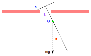 |
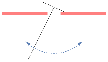
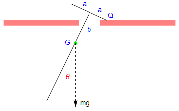
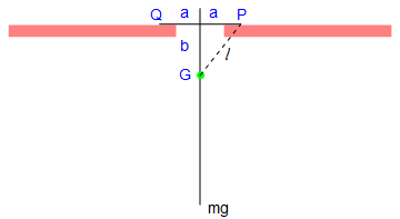
Let the mass of the pendulum be m, and the length of the attached bar be 2 a. Since the construction of the rigid pendulum is symmetric, the center of gyration, which we denote by G, is along the main rod. Let k be the radius of gyration of the pendulum about G, so that the square of its radius of gyration about P and Q is \( k^2 + \ell^2 . \)
The first half-cycle of the motion
Suppose that the pendulum is set in motion from the central position with initial conditions