Preface
This is a tutorial made solely for the purpose of education and it was designed for students taking Applied Math 0330. It is primarily for students who have very little experience or have never used Mathematica before and would like to learn more of the basics for this computer algebra system. As a friendly reminder, don't forget to clear variables in use and/or the kernel.
Finally, the commands in this tutorial are all written in bold black font, while Mathematica output is in normal font. This means that you can copy and paste all commands into Mathematica, change the parameters and run them. You, as the user, are free to use the scripts for your needs to learn the Mathematica program, and have the right to distribute this tutorial and refer to this tutorial as long as this tutorial is accredited appropriately.
Return to computing page for the second course APMA0340
Return to Mathematica tutorial for the second course APMA0330
Return to Mathematica tutorial for the first course APMA0340
Return to the main page for the course APMA0340
Return to the main page for the course APMA0330
Return to Part VI of the course APMA0330
Heaviside function
The Heaviside function was defined previously:
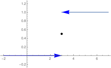
The objective of this section is to show how the Heaviside function can be used to determine the Laplace transforms of piecewise continuous functions. The main tool to achieve this is the shifted Heaviside function H(t-a), where a is arbitrary positive number. So first we plot this function:
b = Graphics[{Blue, Arrowheads[0.07], Arrow[{{3.7, 1}, {3, 1}}]}]
c = Graphics[{Blue, Arrowheads[0.07], Arrow[{{2, 0}, {3, 0}}]}]
d = Graphics[{PointSize[Large], Point[{3, 1/2}]}]
a1 = Graphics[{Blue, Thick, Line[{{-1.99, 0}, {2.9, 0}}]}]
Show[a, a1, b, c, d, PlotRange -> {{-2.1, 7}, {-0.2, 1.2}}]
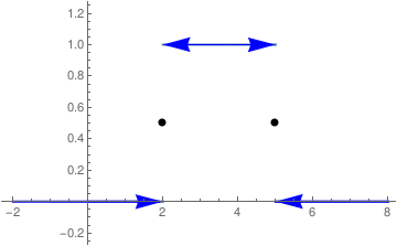
b = Graphics[{Blue, Arrowheads[0.07], Arrow[{{3.7, 1}, {2, 1}}], Arrow[{{3.7, 1}, {5, 1}}]}]
c = Graphics[{Blue, Arrowheads[0.07], Arrow[{{-1, 0}, {2, 0}}]}]
d = Graphics[{PointSize[Large], Point[{2, 1/2}], Point[{5, 1/2}]}]
a1 = Graphics[{Blue, Thick, Line[{{-1.99, 0}, {1.9, 0}}], Line[{{5.01, 0}, {8, 0}}]}]
c2 = Graphics[{Blue, Arrowheads[0.07], Arrow[{{7, 0}, {5, 0}}]}]
Show[a, a1, b, c, c2, d, PlotRange -> {{-2.1, 8}, {-0.2, 1.2}}]
Example: Consider the piecewise continuous function
Dirac delta function
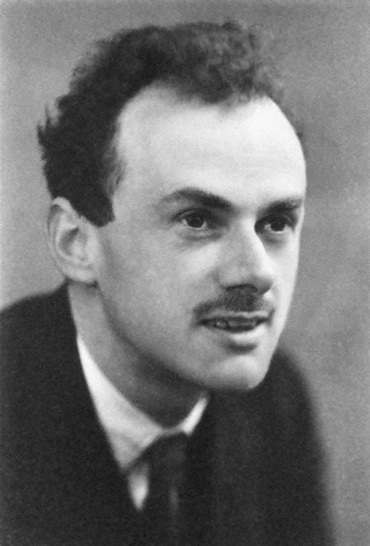
Dirac had traveled extensively and studied at various foreign universities, including Copenhagen, Göttingen, Leyden, Wisconsin, Michigan, and Princeton. In 1937 he married Margit Wigner, of Budapest. Dirac was regarded by his friends and colleagues as unusual in character for his precise and taciturn nature. In a 1926 letter to Paul Ehrenfest, Albert Einstein wrote of Dirac, "This balancing on the dizzying path between genius and madness is awful." Dirac openly criticized the political purpose of religion. He said: "I cannot understand why we idle discussing religion. If we are honest---and scientists have to be---we must admit that religion is a jumble of false assertions, with no basis in reality." He spent the last decade of his life at Florida State University.
The Dirac delta function was introduced as a "convenient notation" by Paul Dirac in his influential 1930 book, "The Principles of Quantum Mechanics," which was based on his most celebrated result on relativistic equation for electron, published in 1928. He called it the "delta function" since he used it as a continuous analogue of the discrete Kronecker delta \( \delta_{n,k} . \) Dirac predicted the existence of positron, which was first observed in 1932. Historically, Paul Dirac used δ-function for modeling the density of an idealized point mass or point charge, as a function that is equal to zero everywhere except for zero and whose integral over the entire real line is equal to one. Dirac’s cautionary remarks (and the efficient simplicity of his idea) notwithstanding, some mathematically well-bred people did from the outset take strong exception to the δ-function. In the vanguard of this group was the American-Hungarian mathematician John von Neumann (was born in Jewish family as János Neumann, 1903--1957), who dismissed the δ-function as a “fiction."
As there is no function that has these properties, the computations that were done by the theoretical physicists appeared to mathematicians as nonsense. It took a while for mathematicians to give strict definition of this phenomenon. In 1938, the Russian mathematician Sergey Sobolev (1908--1989) showed that the Dirac function is a derivative (in generalized sense) of the Heaviside function. To define derivatives of discontinuous functions, Sobolev introduced a new definition of differentiation and the corresponding set of generalized functions that were later called distributions. The French mathematician Laurent-Moïse Schwartz (1915--2002) further extended Sobolev's theory by pioneering the theory of distributions, and he was rewarded the Fields Medal in 1950 for his work. Because of his sympathy for Trotskyism, Schwartz encountered serious problems trying to enter the United States to receive the medal; however, he was ultimately successful. But it was news without major consequence, for Schwartz’ work remained inaccessible to all but the most determined of mathematical physicists.
 |
 |
In 1955, the British applied mathematician George Frederick James Temple (1901--1992) published what he called a “less cumbersome vulgarization” of Schwartz’ theory based on Jan Geniusz Mikusınski's (1913--1987) sequential approach. However, the definition of δ-function can be traced back to the early 1820s due to the work of James Fourier on what we now know as the Fourier integrals. In 1828, the δ-function had intruded for a second time into a physical theory by George Green who noticed that the solution to the nonhomogeneous Poisson equation can be expressed through the solution of a special equation containing the delta function. The history of the theory of distributions can be found in "The Prehistory of the Theory of Distributions" by Jesper Lützen (University of Copenhagen, Denmark), Springer-Verlag, 1982.
Outside of quantum mechanics the delta function is also known in engineering and signal processing as the unit impulse symbol. Mechanical systems and electrical circuits are often acted upon by an external force of large magnitude that acts only for a very short period of time. For example, all strike phenomenon (caused by either piano hammer or tennis racket) involve impulse functions. Also, it is useful to consider discontinuous idealizations, such as the mass density of a point mass, which has a finite amount of mass stuffed inside a single point of space. Therefore, the density must be infinite at that point and zero everywhere else. Delta function can be defined as the derivative of the Heaviside function, which (when formally evaluated) is zero for all \( t \ne 0 , \) and it is undefined at the origin. Now time comes to explain what a generalized function or distribution means.
In our everyday life, we all use functions that we learn from school as a map or transformation of one set (usually called input) into another set (called output, which is usually a set of numbers). For example, when we do our annual physical examinations, the medical staff measure our blood pressure, height, and weight, which all are functions that can be described as nondestructive testing. However, not all functions are as nice as previously mentioned. For instance, a biopsy is much less pleasant option and it is hard to call it a function, unless we label a destructive testing function. Before procedure, we consider a patient as a probe function, but after biopsy when some tissue has been taken from patient's body, we have a completely different person. Therefore, while we get biopsy laboratory results (usually represented in numeric digits), the biopsy represents destructive testing. Now let us turn to another example. Suppose you visit a store and want to purchase a soft drink, i.e. a bottle of soda. You observe that liquid levels in each bottle are different and you wonder whether they filled these bottles with different volumes of soda or the dimensions of each bottle differ from one another. So you decide to measure the volume of soda in a particular bottle. Of course, one can find outside dimensions of a bottle, but to measure the volume of soda inside, there is no other option but to open the bottle. In other words, you have to destroy (modify) the product by opening the bottle. The function of measuring the soda by opening the bottle could represent destructive testing
Now consider an electron. Nobody has ever seen it and we do not know exactly what it looks like. However, we can make some measurements regarding the electron. For example, we can determine its position by observing the point where electron strikes a screen. By doing this we destroy the electron as a particle and convert its energy into visible light to determine its position in space. Such operation would be another example of destructive testing function, because we actually transfer the electron into another matter, and we actually loose it as a particle. Therefore, in real world we have and use nondestructive testing functions that measure items without their termination or modification (as we can measure velocity or voltage). On the other hand, we can measure some items only by completely destroying them or transferring them into another options as destructive testing functions. Mathematically, such measurement could be done by integration (hope you remember the definition from calculus):
Let f(x) be a continuous function that vanishes at infinity. We use integration by parts to evaluate the integral
The definition of the delta function can be extended to piecewise continuous functions:
To understand the behavior of Dirac delta function, we introduce the rectangular pulse function
Labeled[Plot[f[x], {x, 0, 7}, Exclusions -> {False}, PlotStyle -> Thick,
Ticks -> {{{2, "a-1/2h"}, {3, "a+1/2h"}}, {Automatic, {1, "h"}}}], "The pulse function"]
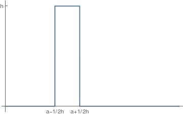
As it can be seen from figure, the amplitude of pulse becomes very large and its width becomes very small as \( h \to \infty . \) Therefore, for any value of h, the integral of the rectangular pulse
Instead of large parameter h, one can choose a small one:
Although the delta function is a distribution (which is a functional on a set of probe functions) and the notation \( \delta (x) \) makes no sense from a mathematician point of view, it is a custom to manipulate the delta function \( \delta (x) \) as with a regular function, keeping in mind that it should be applied to a probe function. Dirac remarks that “There are a number of elementary equations which one can write down about δ-functions. These equations are essentially rules of manipulation for algebraic work involving δ-functions. The meaning of any of these equations is that its two sides give equivalent results [when used] as factors in an integrand.'' Examples of such equations are
Theorem: The convolution of a delta function with a continuous function:
Theorem: The Laplace transform of the Dirac delta function:
Example: Find the Laplace transform of the convolution of the function \( f(t) = t^2 -1 \) with shifted delta function \( \delta (t-3) . \)
According to definition of convolution,
Example: A spring-mass system with mass 1, damping 2, and spring constant 10 is subject to a hammer blow at time t = 0. The blow imparts a total impulse of 1 to the system, which is initially at rest. Find the response of the system. The situation is modeled by
Return to Mathematica page
Return to the main page (APMA0330)
Return to the Part 1 (Plotting)
Return to the Part 2 (First Order ODEs)
Return to the Part 3 (Numerical Methods)
Return to the Part 4 (Second and Higher Order ODEs)
Return to the Part 5 (Series and Recurrences)
Return to the Part 6 (Laplace Transform)
Return to the Part 7 (Boundary Value Problems)