Preface

---

This is a tutorial made solely for the purpose of education and it was designed for students taking Applied Math 0330. It is primarily for students who have very little experience or have never used Mathematica before and would like to learn more of the basics for this computer algebra system. As a friendly reminder, don't forget to clear variables in use and/or the kernel.

Finally, the commands in this tutorial are all written in bold black font, while Mathematica output is in normal font. This means that you can copy and paste all commands into Mathematica, change the parameters and run them. You, as the user, are free to use the scripts for your needs to learn the Mathematica program, and have the right to distribute this tutorial and refer to this tutorial as long as this tutorial is accredited appropriately.

Linear Operators

---

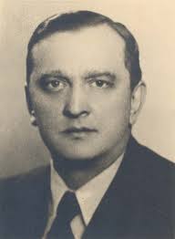
The modern definition of a linear operator was first given by G. Peano for a particular case. However, it was Stefen Banach who defined an operator as a function whose domain is a set of functions. Stefan Banach (1892 – 1945) was a Polish mathematician who is generally considered one of the world's most important and influential 20th-century mathematicians. He was one of the founders of modern functional analysis, and an original member of the Lwów School of Mathematics. When Nazi German troops conquered Lvov in 1941, all institutions of higher education were closed to Poles. The majority of intelligent people (professors, musicians, actors, writers, painters, and many others) were executed, but Banach survived the Nazi slaughter of Polish university professors. Stefan was born in Kraków (then part of the Austro-Hungarian Empire) and passed away in Lvov (Soviet Union) with lung cancer. Stefan was a heavy smoker, and his name was given to one famous probabilistic problem, as well as to many theorems. From 1910 to 1914 and since 1920, he dwelt in Lvov (Lwów, in Polish). At the time Banach studied there, under Austrian control as it had been from the partition of Poland in 1772. In Banach's youth Poland, in some sense, did not exist and Russia controlled much of the country. Banach was given the surname of his mother, who was identified as Katarzyna Banach on his birth certificate, and the first name of his father, Stefan Greczek. He never knew his mother, who vanished from the scene after Stefan was baptized, when he was only four days old, and nothing more is known of her.

In the spring of 1916, Hugo Steinhaus (1887--1972) made a major impact on Banach's life. Stefan wrote his first paper together with Steinhaus. Banach major work was the 1932 book, Théorie des opérations linéaires (Theory of Linear Operations), the first monograph on the general theory of functional analysis. Hugo Steinhaus was a Polish mathematician (of Jewish decent) whose book Mathematical Snapshots has been very influential. Steinhaus obtained his PhD under David Hilbert.

By an operator we mean a transformation that maps a function into another function. A linear operator L is an operator such that \( L[af+bg] = aLf + bLg \) for any functions f, g and any constants a, b. Since we mostly interested in linear differential operators, we need to start with the derivative operator, which we denote by \( \texttt{D} . \) From calculus, we know that the result of application of the derivative operator on a function is its derivative:

We also know that the derivative operator and its inverse, \( \texttt{D}^{-1} = \int , \) are both linear operators. It is easy to construct compositions of derivative operator recursively \( \texttt{D}^{n} = \texttt{D} \left( \texttt{D}^{n-1} \right) , \quad n=1,2,\ldots ,\) and their linear combinations: where coefficients of the above linear differential operator, \( L\left[ x,\texttt{D} \right] , \quad a_n , \ a_{n-1} , \ \ldots , \ a_1, \ a_0 , \) could be either some functions or even constants. Generally speaking, we should multiply the last coefficient a₀ by the identity operator, \( {\bf I} = \texttt{D}^0 , \) but lazy people usually drop it. Since multiplication by the identity operator does not change the result, we can omit it. The leading coefficient a_n is assumed to be not identically zero. In this case we say that the linear differential operator is of the order n.

Let us consider, for simplicity, the case n = 2. With a function y = y(x) that is twice differentiable, we assign another function, which we denote (Ly)(x) (or L[y] or simply Ly). L[y] is the linear differential operator that acts on y(x) by the relation

where \( a_2 (x), \ a_1 (x), \ \mbox{ and } a_0 (x) \) are given functions, and \( a_2 (x) \ne 0. \) In mathematical terminology, L is an operator that operates on functions; that is, there is a prescribed recipe for associating with each function y(x) a new function (Ly)(x). An operator L assigns to each function y(x) having two derivatives a new function called (Ly)(x). Therefore, the concept of an operator coincides with the concept of a ``function of a function.''

With such defined linear differential operator, we can rewrite any linear differential equation in operator form:

If the right-hand term (also called the driving function) is not identically zero, \( f(x) \ne 0 , \) we call the above equation nonhomogeneous (or inhomogeneous). The equation, which is referred to as the homogeneous equation, with an identically zero driving term is of particular interest: The set of all solutions of the homogeneous equation \( L\left[ x,\texttt{D} \right] y =0 \) is called the kernel of the differential operator. In other words, any solution of the above homogeneous linear differential equation belongs to the kernel of the corresponding differential operator.

Example: Let \( L\left[ x,\texttt{D} \right] = \texttt{D} - x^2 \) be a first order linear differential operator (with variable coefficient). Find its kernel, denoted by ker(L).

Solution: Let \( y \in \mbox{ker}(L) , \) then by the definition of the kernel,

Separating variables and integrating, we obtain where C is an arbitrary constant. Therefore, the kernel of the given differential operator consists of all multiples of the exponential function.

Example: Consider the second order Chebyshev differential operator of second kind

where n is a positive integer and \( \texttt{D} \) is the derivative operator, that is, \( \texttt{D} y = y' \quad\mbox{and}\quad \texttt{D}^2 y = y''. \) The corresponding differential equation

is known to have a polynomial solution \( y= U_n ( x ) , \) called the Chebyshev polynomial of the second kind. Mathematica has a dedicated command to define such polynomial: ChebyshevU[x,n]. We find another linearly independent solution using reduction of order. So we seek another solution in the form

Denoting the first derivative of u as v = u', we get the first order separable differential equation Integration yields Next integration gives Therefore, the kernel of the Chebyshev differential operator of the second order is spanned on two functions We summarize our observation in the following theorem:

Theorem: The kernel of a linear differential operator of order n with continuous coefficients in some interval is n-dimensional and it is spanned on n

linearly independent functions \( y_1 (x), \ y_2 (x), \ \ldots , y_n (x) . \) Then any solution of the homogeneous linear differential equation \( L\left[ x,\texttt{D} \right] y =0 \) can be represented as a linear combination of these functions with some constants C₁, ... , C_n ■