Preface
This is a tutorial made solely for the purpose of education and it was designed for students taking Applied Math 0330. It is primarily for students who have very little experience or have never used Mathematica before and would like to learn more of the basics for this computer algebra system. As a friendly reminder, don't forget to clear variables in use and/or the kernel.
Finally, the commands in this tutorial are all written in bold black font, while Mathematica output is in normal font. This means that you can copy and paste all commands into Mathematica, change the parameters and run them. You, as the user, are free to use the scripts for your needs to learn the Mathematica program, and have the right to distribute this tutorial and refer to this tutorial as long as this tutorial is accredited appropriately.
Return to computing page for the second course APMA0340
Return to Mathematica tutorial for the second course APMA0330
Return to Mathematica tutorial for the first course APMA0340
Return to the main page for the course APMA0340
Return to the main page for the course APMA0330
Return to Part IV of the course APMA0330
Padé Approximation
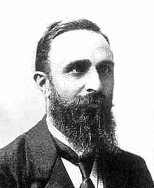
A Padé approximant is the "best" approximation of a function by a rational function of given order -- under this technique, the approximant's power series agrees with the power series of the function it is approximating. The technique was developed around 1890 by the French mathematician Henri Padé (1863--1953), but goes back to the German mathematician Georg Frobenius (1849--1917) who introduced the idea and investigated the features of rational approximations of power series. Henri Eugène Padé, while preparing his doctorate under Charles Hermite, he introduced what is now known as the Padé approximant.
Given a function f and two integers \( m \ge 0 \quad\mbox{and}\quad n \ge 1, \) the Padé approximant of order [m/n] is the rational function
Example: Consider Padé approximants for cosine functions
Return to Mathematica page
Return to the main page (APMA0330)
Return to the Part 1 (Plotting)
Return to the Part 2 (First Order ODEs)
Return to the Part 3 (Numerical Methods)
Return to the Part 4 (Second and Higher Order ODEs)
Return to the Part 5 (Series and Recurrences)
Return to the Part 6 (Laplace Transform)
Return to the Part 7 (Boundary Value Problems)