Theorem: Suppose that f(x,y) is a continuous function defined in some rectangular region

containing the point \( \left( x_0 , y_0 \right) . \) Then there exists a number h (possibly smaller than δ) so that a solution \( y = \phi (x) \) to the initial value problem is defined for \( x \in (x_0 - h , x_0 + h ) . \) ■

This theorem was proved in 1886 by the Italian mathematician Giuseppe Peano (1858--1932). Giuseppe Peano. Giuseppe Peano was a founder of symbolic logic whose interests centred on the foundations of mathematics and on the development of a formal logical language. In 1890 Peano founded the journal Rivista di Matematica, which published its first issue in January 1891. In 1891, Peano started the Formulario Project. It was to be an "Encyclopedia of Mathematics", containing all known formulae and theorems of mathematical science using a standard notation invented by Peano.

In addition to his teaching at the University of Turin, Peano lectured at the Military Academy in Turin in 1886. The following year he discovered, and published, a method for solving systems of linear differential equations using successive approximations. However Émile Picard had independently discovered this method and had credited the German mathematician Hermann Schwarz (1843--1921) with discovering the method first. In 1888 Peano published the book Geometrical Calculus which begins with a chapter on mathematical logic.

Theorem: Let f(y) be a continuous function on the closed interval [a,b] that has one null \( y^{\ast} \in (a,b) , \) namely, \( f(y^{\ast} ) =0 \) and \( f(y) \ne 0 \) for all other points \( y \in (a,b) . \) If the integral

diverges, then the initial value problem for the autonomous differential equation has the unique solution \( y (x) \equiv y^{\ast} . \) If the integral converges, then the initial value problem has multiple solutions.

Theorem: Suppose that f(x,y) is uniformly Lipschitz continuous in y (meaning the Lipschitz constant L in the inequality \( |f(x,y_1 ) - f(x, y_2 )| \le L\,|y_1 - y_2 | \) can be taken independent of x) and continuous in x. Then, for some positive value δ there exists a unique solution \( y = \phi (x) \) to the initial value problem

on the interval \( \left[ x_0 -\delta , x_0 + \delta \right] . \)

Theorem: Let f(x,y) be continuous for all (x,y) in open rectangle \( R= \left\{ (x,y)\,:\, |x-x_0 | < a, \quad |y- y_0 | < b \,\right\} \) and Lipschitz continuous in y, with constant L independent of x. Then there exists a unique solution to the initial value problem

on the interval. Moreover, if z(x) is the solution to the same problem with the initial condition \( z(x_0 ) = z_0 , \) then

Theorem: Suppose that f(x,y) and \( \frac{\partial f}{\partial y} \) are continuous functions defined in some rectangular region

containing the point \( \left( x_0 , y_0 \right) . \) If these functions are bounded in R: for some positive constants M and K, then the initial value problem has a unique solution in the interval

Since the initial value problem \( y' = f(x,y) , \qquad y(x_0 ) = y_0 \) is equivalent to the Volterra integral equation (subject that the slope function f(x,y) and the solution y(x) are continuous functions) this problem has a unique solution that is the limit of the sequence of function \( \left\{ \phi_n (x) \right\}_{n\ge 0} \) that satisfies the recurrence:

Corollary: The continuous dependence of the solutions on the initial conditions holds whenever slope function f satisfies a global Lipschitz condition.

Corollary: If the solution y(x) of the initial value problem \( y' = f(x,y), \ y(x_0 )= y_0 \) has an a priori bound M, i.e., \( |y(x)| \le M \) whenever y(x) exists, then the solution exists for all \( x \in \mathbb{R} . \)

Example. Consider the initial value problem

where the slope function \( f(y) = 2\,\sqrt{y} \) is continuous on infinite interval \( [0, \infty ) \) but not Lipschitz. So according to Peano's theorem, this initial value problem has a solution. Indeed, we can apply Picard's iteration procedure to obtain a solution \( y(x) \equiv 0 . \) On the other hand, since the given differential equation is autonomous, we can separate variables and integrate: where C is an arbitrary constant. Since we consider only positive branch of the square root function, the above formula is valid only when \( x \ge C . \) Therefore, we get a family of solutions (which is also called the general solution) depending on a parameter C: Using Mathematica, we plot some solutions

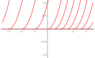
In this sequence of command, I am first entering the family of solutions to the differential equation. Since using C is prohibited in Mathematica, we use CC instead. Then we use two subroutines, one for plotting solutions, and another one for looping with respect to constant C, Finally, we display all graphs.

We can also check that the given initial value problem has multiple solutions by evaluating integral

which converges.

Example. Consider the initial value problem for the Riccati equation

which has a unique solution \( y = \phi (x) \) expressed via Bessel functions This function blows up at \( x \approx 2.003147359 \) --- the first positive root of the transcendent equation \( J_{1/4} \left( \frac{x^2}{2} \right) = Y_{1/4} \left( \frac{x^2}{2} \right) . \) Actually, Picard's theorem guarantees a unique solution within the interval \( \left[ 0, 2^{-1/2} \right] \approx [0,0.707107 ] . \) To find its solution, we use Picard's iteration procedure: and so on.