Return to computing page for the first course APMA0330
Return to computing page for the second course APMA0340
Return to computing page for the fourth course APMA0360
Return to Mathematica tutorial for the first course APMA0330
Return to Mathematica tutorial for the second course APMA0340
Return to Mathematica tutorial for the fourth course APMA0360
Return to the main page for the first course APMA0330
Return to the main page for the second course APMA0340
Return to the main page for the fourth course APMA0360
Return to Part V of the course APMA0340
Introduction to Linear Algebra with Mathematica

Preface


Sturm--Liouville theory is actually a generalization for the infinite dimensional case of famous eigenvalue/eigenvector problems for finite square matrices that we discussed in Part I of this tutorial. Although a Sturm--Liouville problem can be formulated in operator form as L[ y ] = λy similar to the matrix eigenvalue problem Ax = λx, where the operator L is an unbounded differential operator and y is a smooth function.

The corresponding theory that is known as Sturm--Liouville theory originated in two articles by the French mathematician of German descent Jacques Charles François Sturm (1803--1855).
  1. Sturm, J.C.F., "Mémoire sur les Équations différentielles linéaires du second ordre", Journal de Mathématiques Pures et Appliquées, 1836, Vol. 1, pp. 106-186. [sept. 28, 1833]
  2. Sturm, , J.C.F., "Mémoire sur une classe des d'Équations à différences partielles". Journal de Mathématiques Pures et Appliquées, 1836, Vol. 1, pp. 373--444.
Following the same 1836 year, Sturm together with his friend, the French mathematician Joseph Liouville (1809--1882), published very influential articles that provided crucial groundwork for the theory.
  1. Sturm & Liouville, "Démonstration d'un théorème de M. Cauchy relatif aux racines imaginaires des équations". Journal de Mathématiques Pures et Appliquées, 1836, Vol. 1, pp. 278--289.
  2. Sturm & Liouville, "Note sur un théorème de M. Cauchy relatif aux racines des équations simultanées", Comptes rendus de l'Académie des Sciences (English: Proceedings of the Academy of Sciences), 1837, Vol. 4, pp. 720--739.
  3. Sturm & Liouville, "Extrait d'un Mémoire sur le développement des fonctions en séries dont les différents termes sont assujettis à satisfaire à une même équation différentielle lindaire, contenant un paramètre variable", Journal de Mathématiques Pures et Appliquées, 1837, Vol 2, pp. 220--233.
    Comptes rendus de l'Académie des Sciences ((English: Proceedings of the Academy of sciences), 1837, Vol. 4, pp. 675--677.

Sturm--Liouville Problems


Jacques Sturm
A classical Sturm–Liouville theory, named after Jacques Charles François Sturm (1803--1855) and Joseph Liouville (1809--1882), involves analysis of eigenvalues and eigenfunctions for a second order linear differential operator (we use letter L to emphasize that this is a linear operator)
\begin{equation} \label{EqSturm.3} L\left[ x, \texttt{D} \right] = q(x)\,\texttt{I} - \texttt{D}\,p(x)\,\texttt{D} , \qquad \texttt{D} = \frac{\text d}{{\text d}x} , \quad \texttt{I} = \texttt{D}^0 , \end{equation}
where I is the identity operator, and p(x) and q(x) are given continuous functions on some interval [𝑎, b]. Since p(x) follows the derivative operator, it should be a differentiable function, which we abbreviate as p(x) ∈ C¹[𝑎, b]. The linear self-adjoint operator \eqref{EqSturm.3} is referred to as the Sturm--Liouville operator.

Correspondingly, the Sturm--Liouville theory is about a real second-order homogeneous linear self-adjoint differential equation with a parameter λ of the form

\begin{equation} \label{EqSturm.1} \frac{\text d}{{\text d}x} \left[ p(x)\,\frac{{\text d}y}{{\text d}x} \right] - q(x)\, y + \lambda \,w (x)\,y(x) =0 , \qquad a < x < b , \end{equation}
subject to the homogeneous boundary conditions of the third kind
\begin{equation} \label{EqSturm.2} \alpha_0 y(a) - \alpha_1 y'(a) =0 , \qquad \beta_0 y(b ) + \beta_1 y' (b) =0 , \qquad |\alpha_0 | + |\alpha_1 | \ne 0 \quad\mbox{and} \quad |\beta_0 | + |\beta_1 | \ne 0. \end{equation}
There are known some particular important cases:
\begin{align*} & u(a) =0, \quad u(b) = 0 \qquad (\mbox{Dirichlet conditions}); \\ & u' (a) = 0, \quad u'(b) = 0 \qquad (\mbox{Neumann conditions}); \\ & u' (a) , \quad u(b) = 0 \qquad\mbox{or} \qquad u (a) , \quad u'(b) = 0 \qquad (\mbox{mixed conditions}). \end{align*}

An operator L acting in a Hilbert space with inner product ⟨· , ·⟩ is called self-adjoint iff
\[ \langle L\,u , v \rangle = \langle u , L\,v \rangle \]
for every pair of vectors u, v from the domain of operator L.
Note: If boundary conditions \eqref{EqSturm.2} are not homogeneous, Sturm--Liouville theory is not applicable because the set of functions that satisfy these conditions is not a vector space. These two-point boundary value problems \eqref{EqSturm.1}, \eqref{EqSturm.2} occur in many mathematical applications.

Here y = y(x) is a nontrivial (meaning not identically zero) function of the free variable x∈[𝑎, b]. A positive function w(x) is called the "weight" or "density" function---it is not a part of the differential operator \eqref{EqSturm.3}. On the other hand, functions p(x), p'(x), and q(x) are specified at the outset. In the simplest of cases, all coefficients are continuous on the finite closed interval [𝑎, b], and p(x) has continuous derivative. In this simplest case, a nontrivial function y(x) is called a solution of Eq.\eqref{EqSturm.1} if it is twice continuously differentiable on (𝑎, b) and satisfies the given equation at every point in (𝑎, b).

Lemma 1: Any second order differential operator \( a(x)\,\texttt{D}^2 + b(x)\,\texttt{D} \) can be transferred to a self-adjoint form upon multiplying it by an integrating factor:
\[ \mu (x)\,a(x)\,\frac{{\text d}^2 y}{{\text d}x^2} + \mu (x)\, b(x)\,\frac{{\text d}y}{{\text d}x} = \frac{\text d}{{\text d}x} \left( y(x)\, \exp \left\{ \int \frac{b(x)}{a(x)}\,{\text d}x \right\} \right) , \qquad\mbox{with} \qquad \mu (x) = \frac{1}{a(x)}\,\exp \left\{ \int \frac{b(x)}{a(x)}\,{\text d}x \right\} \]
Let us consider an arbitrary second order differential equation
\[ M\left[ x, \texttt{D} \right] u = a(x)\,u'' + b(x)\, u' + c(x)\, u = 0 , \]
with some given continuous functions 𝑎(x), b(x), and c(x). We denote by μ(x) an integrating factor that reduces the differential operator M into exact form:
\[ \mu (x)\,M\left[ x, \texttt{D} \right] y = p(x)\, y'' + p' y' + c(x)\, y . \]
Hence, we get two equations
\[ \mu (x)\,a (c) = p(x), \qquad \mu (x)\,b(x) = p' (x) = \mu' a + \mu \,a' . \]
This yields the differential equation (which is separable) for the integrating factor:
\[ \frac{{\text d}\mu}{{\text d}x} = \mu \left[ b - a' \right] /a \qquad \Longrightarrow \qquad \mu (x) = \exp \left\{ \int \frac{b - a'}{a} \,{\text d} x \right\} . \]
This gives
\[ \mu (x) = \frac{1}{a(x)} \exp \left\{ \int \frac{b}{a}\,{\text d} x \right\} . \]
Therefore, multiplication my μ yields the exact equation:
\[ \mu \left[ a(x)\,y'' + b(x)\,y' \right] = \frac{\text d}{{\text d}x} \left( \exp \left\{ \int \frac{b}{a}\,{\text d} x \right\} \frac{{\text d}y}{{\text d}x} \right) . \]
Lemma 2: Any second order differential equation \( a(x)\,y'' + b(x)\,y' + c(x)\, y =0 \) can be transferred to a normal form upon suitable substitution:
\[ u'' + q(x)\,u =0 . \]
We make the Bernoulli substitution \( y = u(x)\,v(x) . \) Then its derivatives become
\[ y' = u' v + u\,v' , \qquad y'' = u'' v + 2 u' v' + u\, v'' . \]
Substitution of these relations into the given differential equation yields
\[ a(x) \left[ u'' v + 2 u' v' + u\, v'' \right] + b(x) \left[ u' v + u\,v' \right] + c(x)\,u\,v = 0. \]
Upon setting the coefficient of u′ equal to zero and solving, we find that
\[ 2a\, v' + b(x)\, v = 0 \qquad \Longrightarrow \qquad \frac{v'}{v} = - \frac{b(x)}{2\,a(x)} . \]
Integration yields
\[ \ln |v| = - \int \frac{b(x)}{2\,a(x)}\, {\text d}x \qquad \Longrightarrow v(x) = \exp \left\{ - \int \frac{b(x)}{2\,a(x)}\, {\text d}x \right\} . \]
Therefore, the Bernoulli substitution \( y = u(x)\,v(x) \) with
\[ v(x) = \exp \left\{ - \int \frac{b(x)}{2\,a(x)}\, {\text d}x \right\} \]
reduces the differential equation \( a(x)\, y'' + b(x)\, y' + c(x)\,y = 0 \) to the equation in normal form \( u'' + q(x)\,u = 0 \) with
\[ q(x) = \frac{1}{a(x)\,v} \left[ v'' + b(x)\, v' + c(x)\, v \right] . \]
Remark: Transformation of arbitrary differential operator of second order into an operator in self-adjoint form \( L\left[ x, \texttt{D} \right] = q(x)\,\texttt{I} - \texttt{D}\,p(x)\,\texttt{D} \) by means of an integrating factor is not unique---there are known many other options. It is a part of general approach of factorization of differential operator, discussed in tutorial I.

Integration by parts yields
\begin{align*} \left\langle L\,u, v \right\rangle &= \int_a^b q(x)\,u(x)\,v(x)\,{\text d}x - \left. p(x)\,\frac{{\text d}u}{{\text d}x}\, v(x) \right\vert_{x=a}^{x=b} + \int_a^b p(x)\,\frac{{\text d}u}{{\text d}x}\, \frac{{\text d}v}{{\text d}x}\, {\text d} x \\ &= \int_a^b q(x)\,u(x)\,v(x)\,{\text d}x + \int_a^b u(x)\,\frac{\text d}{{\text d}x} \left( p(x)\,\frac{{\text d}v}{{\text d}x} \right) {\text d} x \\ &= \left\langle u, L\,v \right\rangle \end{align*}
because out of integration terms vanish:
\[ - \left. p(x)\,\frac{{\text d}u}{{\text d}x}\, v(x) \right\vert_{x=a}^{x=b} + \left. u(x)\, p(x)\,\frac{{\text d}v}{{\text d}x} \right\vert_{x=a}^{x=b} =0 \]
due to boundary conditions \eqref{EqSturm.2}.


However, the first order differential operator is not self-adjoint independently what boundary conditions cab be imposed. Indeed,
\begin{align*} \left\langle \texttt{D}\,u, v \right\rangle &= \int_a^b u' (x)\,v(x)\,{\text d} x = \left. u (x)\,v(x) \right\vert_{x=a}^{x=b} - \int_a^b u (x)\,v' (x)\,{\text d} x \\ &= u(b) \,v(b) - u(a)\,v(a) - \left\langle u, \texttt{D}\,v \right\rangle . \end{align*}

On the other hand, multiplying the derivative operator by imaginary unity, we obtain the first order differential operator

\[ L_1 \left[ x, \texttt{D} \right] = - {\bf j}\,\texttt{D} = - {\bf j}\,\frac{\text d}{{\text d}x} \]
that is a self-adjoint operator with, for instance, Dirichlet or Neumann boundary conditions
\[ u(a) = u(b) =0 \qquad\mbox{or} \qquad u' (a) = u' (b) =0 , \]
as well as some other boundary conditions (including periodic conditions). Indeed,
\begin{align*} \left\langle -{\bf j}\,\texttt{D}\,u, v \right\rangle &= -{\bf j} \int_a^b u' (x)\,v(x)\,{\text d} x = -{\bf j} \left. u (x)\,v(x) \right\vert_{x=a}^{x=b} +{\bf j} \int_a^b u (x)\,v' (x)\,{\text d} x \\ &= {\bf j} \left[ u(a)\,v(a) - u(b)\,v(b) \right] + \left\langle u, -{\bf j}\,\texttt{D}\,v \right\rangle . \end{align*}

Example 1: Let us consider a constant coefficient differential operator

\[ L\left[ \texttt{D} \right] = \texttt{D}^2 + 5\,\texttt{D} + 4\,\texttt{I} , \qquad \texttt{I} = \texttt{D}^0 . \tag{1.1} \]
Differential operator (1.1) is not self-adjoint; indeed,
\begin{align*} \left\langle L[u], v \right\rangle &= \int_a^b \left( u'' + 5\,u' + 4\,u \right) v(x)\,{\text d}x \end{align*}
Integration by parts yields
\begin{align*} \left\langle L[u], v \right\rangle &= \left( u' v + 5\,u\,v \right)_{x=a}^{x=b} - \int_a^b \left( u' v' + 5\,u\,v' \right) v(x)\,{\text d}x + 4 \int_a^b u(x)\,v(x)\,{\text d}x \\ &= \left( u' v + 5\,u\,v - u\,v' \right)_{x=a}^{x=b} + \int_a^b u(x) \left( v'' -5\,v' + 4\,v \right) {\text d} x \\ &= \left\langle u, L^{\ast} [v] \right\rangle + \left( u' v + 5\,u\,v - u\,v' \right)_{x=a}^{x=b} , \end{align*}
where
\[ L^{\ast} \left[ \texttt{D} \right] = \texttt{D}^2 - 5\,\texttt{D} + 4\, \texttt{I} . \]
Since LL*, the given operator (1.1) is not self-adjoint.

We convert operator (1.1) into self-adjoint form by applying an integrating factor. With 𝑎(x) = 1 and b(x) = 5, we can identify the integrating factor using Lemma 1. Upon multiplication by the integrating factor \( \mu = e^{5x}, \) we reduce the given differential operator to a self-adjoint form:

\[ e^{5x} L \left[ \texttt{D} \right] = e^{5x} \left[ \texttt{D}^2 + 5\, \texttt{D} + 4\,\texttt{I} \right] = \frac{\text d}{{\text d}x} \left( e^{5x} \frac{\text d}{{\text d}x} \right) + 4\, e^{5x} \texttt{I} . \tag{1.2} \]


We can also transfer the same differential operator into self-adjoint form in different way. First, we observe that
\[ \texttt{D}\, e^{ax} u(x) = e^{ax} \left( \texttt{D} + a\,\texttt{I} \right) u \qquad \Longrightarrow \qquad \left( \texttt{D} + a\,\texttt{I} \right) u = e^{-ax} \texttt{D}\, e^{ax} u(x) \tag{1.3} \]
for any constant 𝑎. Since the given differential operator can be factors into a product of first order linear operators
\[ L\left[ \texttt{D} \right] = \texttt{D}^2 + 5\,\texttt{D} + 4\,\texttt{I} = \left( \texttt{D} + 4 \texttt{I} \right) \left( \texttt{D} + \texttt{I} \right) , \]
we obtain
\[ L\left[ \texttt{D} \right] y = e^{-4x} \texttt{D} e^{3x} \texttt{D}\, \left( e^x y \right) , \]
which gives the self-adjoint operator for function \( u(x) = e^x y . \) Hence, the operator L can be written as
\[ L\left[ \texttt{D} \right] y = M\left[ \texttt{D} \right] u = e^{-4x} \texttt{D} e^{3x} \texttt{D} \left( u \right) , \]
including a free term.

Example 2: Let us consider a variable coefficient differential operator

\[ L\left[ \texttt{D} \right] = x^2 \texttt{D}^2 + 3x\, \texttt{D} - 3\,\texttt{I} , \qquad \texttt{I} = \texttt{D}^0 . \tag{2.1} \]
This operator is not self-adjoint. To show this, we consider every its term separately. For the second derivative term, we have
\begin{align*} \left\langle x^2 u'' , v \right\rangle &= \left( x^2 u' v \right)_{x=a}^{x=b} - \int_a^b u' \left( 2x\,v + x^2 v' \right) {\text d}x \\ &= \left( x^2 u' v - 2x\,v' u - x^2 u\, v' \right)_{x=a}^{x=b} + \int_a^b u \left( x^2 v'' + 4x\,v' + 2\,v \right) {\text d}x . \end{align*}
For the second term, we have
\[ \left\langle x\, u' , v \right\rangle = \left( x\,uv \right)_{x=a}^{x=b} - \int_a^b u \left( v + x\,v' \right) {\text d}x . \]
Combining all terms together, we get
\begin{align*} \left\langle L[ x, \texttt{D} ]\,u , v \right\rangle &= \left( x^2 u' v - 2x\,v' u - x^2 u\, v' + 3x\,uv \right)_{x=a}^{x=b} + \int_a^b u \left( x^2 v'' + 4x\,v' + 2\,v - 3v - 3x\,v' + 3v \right) {\text d}x \\ &= \left( x^2 u' v - 2x\,v' u - x^2 u\, v' + 3x\,uv \right)_{x=a}^{x=b} + \left\langle u, L^{\ast} \left[ x, \texttt{D} \right] v \right\rangle , \end{align*}
where
\[ L^{\ast} \left[ x, \texttt{D} \right] = x^2 \texttt{D}^2 + x\,\texttt{D} + 2\,\texttt{I} . \]
Since LL*, the given operator (1.1) is not self-adjoint.

To convert operator (2.1) into a self-adjoint form, we find an integrating factor; using Lemma 1, we identify 𝑎(x) = x², b(x) = 3x, and c = −3. Then

\[ \mu (x) = \frac{1}{a(x)}\,\exp \left\{ \int \frac{b(x)}{a(x)}\,{\text d}x \right\} = \frac{1}{x^2} \,\exp \left\{ \int \frac{3x}{x^2}\,{\text d}x \right\} = x . \]
So multiplication by x yields
\[ x\,L\left[ \texttt{D} \right] = x^3 \texttt{D}^2 + 3x^2 \texttt{D} - 3x\,\texttt{I} = \texttt{D}\, x^3 \texttt{D} - 3x\,\texttt{I} , \]
which is in self-adjoint form.
End of Example 2

Upon introducing boundary operators

\begin{equation} \label{EqSturm.4} B_a y = \alpha_0 y(a) - \alpha_1 y'(a) \qquad\mbox{and}\qquad B_{b} y = \beta_0 y(b) + \beta_1 y' (b) , \end{equation}
we can rewrite this Sturm--Liouville problem in operator form:
\begin{equation} \label{EqSturm.5} L\left[ x, \texttt{D} \right] y = w\,\lambda y , \qquad B_a y = 0, \quad B_{b} y = 0. \end{equation}
This boundary value problem has an obvious solution---the identically zero function. Since we are not after such a trivial solution, we need something more. The Sturm--Liouville problem (S-L, for short) consists of two parts: the first part is about finding values of parameter λ for which the problem has a nontrivial solution (not identically zero); such values are called eigenvalues. The second part includes determination of nontrivial solutions that are called eigenfunctions. Note that a Sturm--Liouville problem may have other constraints, not necessarily formulated above.

A Sturm--Liouville problem consists of a differential equation with a parameter (usually denoted by λ) subject to some additional conditions. These additional conditions could be homogeneous boundary conditions, periodic conditions or of some other type. The Sturm--Liouville problem involves finding nontrivial (not identically zero) solutions, called eigenfunctions and corresponding values of parameter λ, called eigenvalues. The set of all eigenvalues is called spectrum of the Sturm--Liouville problem. The pairof eigenvalue λ and corresponding eigenfunction u>, (λ, u), is called an eigenpair for the Sturm--Liouville problem \eqref{EqSturm.1}, \eqref{EqSturm.2}.

The theory of Sturm--Liouville problems is well developed for second order differential equations. The most complete part of it is devoted to self-adjoint differential operators \eqref{EqSturm.3}, which is our objective. However, many results are known for not self-adjoint problems, problems with parameter λ in boundary conditions, and equations of order higher than two. It should be noted that spectrum for forth order (and higher) differential equations may have very complicated.

There are two kinds of Sturm--Liouville problems for second order differential operators. One is called classical or regular when p(x) > 0 and 1/p(x) > 0 for all points from the closed interval x∈[𝑎, b]. These assumptions are necessary to render the theory as simple as possible while retaining considerable generality. It turns out that these conditions are valid in many problems that we will consider shortly. If p(𝑎) = 0, or p(b) = 0, or p(𝑎) = 0 = p(b), the Sturm--Liouville problem is said to be singular. If conditions on coefficients p(x), q(x), and ρ(x) are held to make the Sturm--Liouville problem regular, but the interval is unbounded, then such problem is also referred to as singular.

Theorem 1: If p(x) > 0, q(x) > 0, and \( \left. p\,u\,u' \right\vert_{x=a}^{x=b} \leqslant 0, \) then classical Sturm--Liouville operator \eqref{EqSturm.3} is positive meaning that all its eigenvalues are positive. If q(x) ≥ 0, then its spectrum is nonnegative.
Let u be an eigenfunction corresponding to an eigenvalue λ for a classical Sturm--Liouville operator \eqref{EqSturm.3}. This means that u belongs to the domain of the operator \( L\left[ x, \texttt{D} \right] = q(x) \texttt{I} - \texttt{D}\,p(x)\,\texttt{D} , \) so u(x) is twice continuously differentiable and satisfies the homogeneous boundary conditions \eqref{EqSturm.2}. Then
\begin{align*} \langle u, L\,u \rangle &= \langle u, \lambda\,u \rangle = \lambda\,\langle u, u \rangle = \lambda \,\| u \|^2 \\ &= \int_a^b \left( q\,u^2 - u\,\texttt{D}\,p(x)\,\texttt{D} \,u \right) {\text d}x . \end{align*}
Integration by parts yields
\[ - \int_a^b u\,\texttt{D}\,p(x)\,\texttt{D} \,u \, {\text d}x = -\left. u(x)\,p(x) \,\frac{{\text d}u}{{\text d}x} \right\vert_{x=a}^{x=b} + \int_a^b p(x) \left( \frac{{\text d}u}{{\text d}x} \right)^2 {\text d}x . \]
This gives
\[ \lambda \,\| u \|^2 = -\left. u(x)\,p(x) \,\frac{{\text d}u}{{\text d}x} \right\vert_{x=a}^{x=b} + \int_a^b p(x) \left( \frac{{\text d}u}{{\text d}x} \right)^2 {\text d}x > 0 \]
according to the condition in Theorem 1.
Joseph Liouville
Jacques Charles François Sturm (1803--1855) was a French mathematician of Switzerland descent. Charles spent his adult life in Paris. His primary interests were fluid mechanics and differential equations. Sturm along with the Swiss engineer Daniel Colladon was the first to accurately determine the speed of sound in water. In mathematics, he won the coveted Grand prix des Scienes Mathematiques for his work in differential equations. Sturm held the chair of mechanics at the Sorbonne and was elected a member of the French Academy of Sciences. The asteroid 31043 Sturm is named for him. Sturm's name is one of the 72 names engraved at the Eiffel Tower.

Joseph Liouville was a French mathematician known for his work in analysis, differential geometry, and number theory and for his discovery of transcendental numbers---i.e., numbers that are not the roots of algebraic equations having rational coefficients. He was also influential as a journal editor and teacher. Joseph founded the Journal de Mathématiques Pures et Appliquées which retains its high reputation up to today.

In physics and other applications, many problems arise in the form of boundary value problems involving second order ordinary differential equations, written in self-adjoint form:

\[ L\left[ x, \texttt{D} \right] = q(x)\, \texttt{I} -\texttt{D} \left( p(x)\,\texttt{D} \right) \qquad \mbox{or}\qquad L\left[ x, \texttt{D} \right] y = q(x) \, y -\frac{\text d}{{\text d}x} \left( p(x)\,\frac{{\text d}y}{{\text d}x}\right) , \]
where \( \texttt{D} = {\text d}/{\text d}x \) is the derivative operator and \( \texttt{I} = \texttt{D}^0 \) is the identity operator. Sturm was the first who generalized the well known matrix problem for eigenvalues/eigenvectors to the linear differential operators by considering the eigenvalue problem \eqref{EqSturm.5} for functions y(x) subject to some boundary conditions. Now this problem is referred to as the Sturm--Liouville problem. Here p(x), q(x), and ρ(x) > 0 are specified continuous functions at the outset, which is usually some interval (finite or not) of real axis ℝ.

Example 3: Let us consider the simplest self-adjoint differential operator with q = 0:

\[ L\left[ \texttt{D} \right] = - \texttt{D}^2 \qquad\mbox{on interval}\quad (0, \ell ) , \qquad \ell > 0. \]
We analyze several eigenvalue/eigenfunction problems for this differential operator subject to different boundary conditions.


Example 3D (Dirichlet boundary conditions): Let us consider the one-dimensional Schrödinger equation

\[ - \frac{\hbar}{2m}\,\psi'' (x) = E\, \psi (x) , \qquad x \in (0, \ell ) , \]
subject to the first kind boundary conditions, also known as Dirichlet boundary conditions:
\[ \psi (0) = 0 \qquad \psi (\ell ) = 0 . \]
When a function is specified at the boundary, then the corresponding boundary conditions are named after G. Dirichlet. We rewrite the corresponding Sturm--Liouville problem (SL problem for short) in the standard form by setting λ = 2m E/ ℏ:
\[ y'' + \lambda \,y =0 , \qquad y(0) = 0, \quad y(\ell ) =0 . \tag{3D.1} \]
First, we need to find the general solution to the SL equation in (3D.1). It depends on the roots of the characteristic equation:
\[ r^2 + \lambda = 0 \qquad \Longrightarrow \qquad r = \pm \sqrt{-\lambda} . \tag{3D.2} \]
Solutions of the differential equation \( y'' + \lambda \,y =0 \) depend on the sign of parameter λ. When λ = −μ² is negative, the general solution is a linear combination of two exponential terms
\[ y (x) = c_1\, e^{\sqrt{-\lambda}\,x} + c_2\, e^{\sqrt{-\lambda}\,x} , \]
with some arbitrary constants c₁ and c₂. From the first boundary condition at the origin, we have
\[ y(0) = c_1 + c_2 =0 \qquad \Longrightarrow \qquad c_1 = - c_2 . \]
The boundary condition at x = ℓ dictates
\[ y(\ell ) = c_1 \left( e^{\mu \ell} - e^{-\mu \ell} \right) = 2\,c_1 \sinh (\mu \ell) =0 . \]
Since sine hyperbolic can be zero only at the origin, we conclude that negative value of λ cannot be an eigenvalue.

If λ =0, the general solution of the differential equation \( y'' =0 \) is a linear function:

\[ y(x) = c_1 + c_2 x . \]
From boundary conditions, it follows
\[ y(0) = c_1 =0 \qquad\mbox{and} \qquad y(\ell ) = c_2 \ell =0 . \]
So for λ =0 there is no nontrivial solution.

For positive λ = ω2, we get two linearly independent solutions sin (ωx) and cos (ωx), so their linear combination gives us the general solution.

\[ y(x) = c_1 \cos (\omega x) + c_2 \sin (\omega x) . \]
To satisfy the boundary conditions, we have to fulfill the equations
\[ y(0) = c_1 = 0 \qquad \mbox{and} \qquad y(\ell ) = c_2 \sin (\omega\ell ) =0 . \]
in order for function y to be other than zero, we must choose ω as
\[ \omega = \sqrt{\lambda} = \frac{n\pi}{\ell} , \qquad n=1,2,3,\ldots . \]
Therefore, we get the eigenvalues
\[ \lambda_n = \left( \frac{n\pi}{\ell} \right)^2 \qquad \Longrightarrow \qquad E_n = \frac{1}{2m} \left( \frac{\hbar \pi n}{\ell} \right)^2 , \qquad n=1,2,3,\ldots ; \]
and corresponding eigenfunctions:
\[ \phi_n (x) = \sin \left( \frac{n\pi x}{\ell} \right) , \qquad n=1,2,3,\ldots . \]


Rayleigh quotient:

Let us pretend that we don’t know the eigenpairs. Upon writing the equation for a particular eigenvalue λn with corresponding eigenfunction ϕn, we get

\[ \phi''_n + \lambda_n \phi_n = 0, \qquad \phi_n (0) = \phi_n (\ell ) = 0. \]
Now multiply by ϕn and integrate over the given interval
\[ \int_a^b \phi_n \phi''_n {\text d}x + \lambda_n \int_a^b \left( \phi_n \right)^2 {\text d}x = 0, \]
We integrate the first integral by parts to obtain:
\[ \left. \phi_n (x)\,\phi'_n (x) \right\vert_{x=a}^{x=b} - \int_a^b \left( \phi'_n \right)^2 {\text d}x . \]
The first terms vanish because of the boundary conditions. We substitute the result above into the equation and rearrange it to yield
\[ \lambda_n = \dfrac{\langle \phi_n , -\phi''_n \rangle}{\langle \phi_n , \phi_n \rangle} = \dfrac{\int_a^b \left( \phi'_n \right)^2 {\text d}x}{\int_a^b \left( \phi_n \right)^2 {\text d}x} . \]
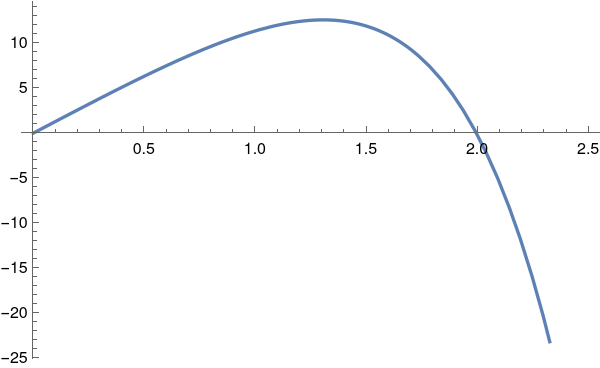
The goal is to estimate the eigenvalue λn without actually solving the differential equation, analytically or numerically. Let’s suppose that we wish to estimate the lowest eigenvalue λ₁, known as the principal eigenvalue. We’ll consider the special case ℓ = 2. he exact answer is \( \lambda_1 = \left( \frac{\pi}{\ell} \right)^2 . \) When ℓ = 2, it is
N[(Pi/2)^2]
2.4674
If we take \( u(x) = x(x-2) \) to satisfy the Dirichlet boundary conditions, then its Rayleigh quotient becomes
\[ R[u] = \frac{\langle u, L\,u \rangle}{\langle u, u \rangle} = \frac{F[u]}{\| u \|^2} = 2.5 . \]
with
\[ F[u] = \langle u, L\,u \rangle = \int_0^2 (u')^2 \,{\text d}x = \int_0^2 \left( 2x -2 \right)^2 {\text d} x = \frac{8}{3} , \]
\[ \langle u, u \rangle = \| u \|^2 = \int_0^2 x^2 (x-2)^2 {\text d}x = \frac{16}{15} . \]
2* Integrate[(2*x - 2)^2, {x, 0, 2}]
8/3
Integrate[x*x*(x - 2)^2, {x, 0, 2}]
16/15
8/3/(16/15)
5/2
So we see that 2.5 is larger than the principal eigenvalue, λ₁ ≈ 2.4674;. Since we are trying to estimate the lowest eigenvalue, we’ll use functions that have no zeroes in (0,1) – the idea is to use a function that approximates the eigenfunction ϕ₁(x). We’ll try several functions, and denote each one as ut(x) for “trial function”, or simply u(x). Another trial function can be chosen as
\[ u(x) = \begin{cases} x, & \ \mbox{ for }\quad 0 < x < 1, \\ 2-x , & \ \mbox{ for }\quad 1 < x < 2. \end{cases} \]
Note that the derivative of this trial function is ±1 for x ≠ 1. As such, the numerator of the Rayleigh quotient becomes
\[ \int_0^2 \left( u' \right)^2 {\text d} x = \int_0^2 {\text d} x = 2. \]
The denominator is
\[ \int_0^2 \left( u \right)^2 {\text d} x = \int_0^1 x^2 {\text d} x + \int_1^2 \left( 2 -x \right)^2 {\text d} x = \frac{1}{3} + \frac{1}{3} = \frac{2}{3} . \]
Therefore, the Rayleigh quotient associated with this trial function, has value 3, which lies above the true value λ₁ ≈ 2.4674;.

However, if we take as a trial function u = sin(πx/2), the Rayleigh quotient for this function becomes

\[ R[u] = \dfrac{\int_0^2 \left( u' \right)^2 {\text d}x}{\int_0^2 \left( u \right)^2 {\text d}x} = \frac{\pi^2}{4} \cdot \dfrac{\int_0^2 \left( \cos (\pi x/2) \right)^2 {\text d}x}{\int_0^2 \left( \sin (\pi x/2) \right)^2 {\text d}x} = \frac{\pi^2}{4} , \]
which is the exact value of lowest eigenvalue λ₁.


Now we consider another function
\[ u(x) = x \left( x-1 \right) \left( x-2 \right) , \]
which has one node at x = 1. Hence, we expect that this trial function will peovide a good approximation for ϕ₂(x) = sin(πx), the eigenfunction corresponding to the second eigenvalue λ₂ = π² ≈ 9.8696.

Using Mathematica, we find the Rayleigh quotient for this trial function:

u[x_] = x*(x - 1)*(x - 2);
Integrate[(D[u[x], x])^2, {x, 0, 2}]
8/5
Integrate[(u[x])^2, {x, 0, 2}]
16/105
8/5*105/16
21/2
\[ R[u] = \dfrac{\int_0^2 \left( u' \right)^2 {\text d}x}{\int_0^2 \left( u \right)^2 {\text d}x} = \frac{21}{2} =10.5, \qquad u(x) = x \left( x-1 \right) \left( x-2 \right) . \]
This is a good approximation to the second eigenvalue λ₂ = π² ≈ 9.8696.    ■

Example 3N (Neumann boundary conditions): We consider a similar Sturm--Liouville problem (SL for short), but with the second kind boundary conditions, also known as Neumann boundary conditions:

\[ y'' + \lambda \,y =0 , \qquad y'(0) = 0, \quad y'(\ell ) =0 . \]
As usual, prime stands for the derivative (in Lagranhe notation), y' = dy/dx. It could be shown similarly to the previous example that negative λ are not possible. So we need to consider only two cases: λ = 0 and λ = ω² > 0. The former gives us an eigenvalue λ = 0 to which corresponds a constant as an eigenfunction. To the latter corresponds the general solution
\[ y(x) = c_1 \cos (\omega x) + c_2 \sin (\omega x) \qquad \Longrightarrow \qquad y' (x) = \omega \left[ -c_1 \sin (\omega x) + c_2 \cos (\omega x) \right] . \]
The boundary conditions dictate c₂ = 0 and \( \sin (\omega \ell ) =0 . \) Thus, we get eigenvalues and corresponding eigenfunctions
\[ \lambda_n = \left( \frac{n\pi}{\ell} \right)^2 , \qquad y_n (x) = \cos\left( \frac{n\pi x}{\ell} \right) , \qquad n=0,1,2,\ldots . \]
The principal eigenvalue is λ0 = 0. Let us take a function that satisfies the Neumann boundary conditions (we choose ℓ = 2):
\[ u(x) = x^2 (x-2)^2 . \]
Its Rayleigh quotient is
\[ R[u] = \frac{\langle u, L\,u \rangle}{\langle u, u \rangle} = 3 \]
with
\[ \langle u, L\,u \rangle = 2\int_0^2 x^2 (x-2)^2 \left( -8 + 24 x - 12 x^2 \right) {\text d}x = \frac{256}{105} \qquad \langle u, u \rangle = \int_0^2 x^4 (x-2)^4 {\text d}x = \frac{256}{315} . \]
u[x_] = x^2 *(x - 2)^2;
Integrate[-u[x]*D[u[x], x, x], {x, 0, 2}]
256/105
Integrate[u[x]*u[x], {x, 0, 2}]
256/315
256/105/(256/315)
3
That is, the Rayleigh quotient yields an upper bound 3.0 of the principal eigenvalue. λ0 = 0, and also the next eigenvalue λ₁ = π²/4 ≈ 2.4674.


Now suppose we choose another trial function
\[ u(x) = \begin{cases} 1, & \quad\mbox{if} \quad 0 < x < 1, \\ (2-x)^2 , & \quad\mbox{if} \quad 1 < x < 2. \end{cases} \]
The functional in the numerator of the Rayleigh quotient \eqref{EqSturm.8} is
\[ F[u] = \int_0^2 \left( u' \right)^2 {\text d} x = 4 \int_1^2 (2-x)^2 {\text d} x = \frac{4}{3} . \]
The norm squared is
\[ \| u \|^2 = \int_0^2 \left( u \right)^2 {\text d} x = \int_0^1 {\text d}x + \int_1^2 (2-x)^4 {\text d} x = \frac{6}{5} . \]
Thus, the Rayleigh quotient gives an upper estimate of
\[ R[u] = \frac{F[u]}{\| u \|^2} = \frac{10}{9} \approx 1.11111 \]
to the lowest eigenvalue λ0 = 0. However, any constant trial function will give the true value of λ0 = 0.    ■

Example 3M: There are two known Sturm--Liouville problems with mixed boundary conditions when on one end we have the Dirichlet condition while on the other end we have the Neumann condition. So we start with one of them:

\[ y'' + \lambda \,y =0 , \qquad y(0) = 0, \quad y'(\ell ) =0 . \]
It is clear from our previous discussion that eigenvalues must be positive in the given Sturm--Liouville problem. The general solution (λ > 0) of the equation \( y'' + \lambda \,y = 0 \) subject to the Dirichlet boundary condition at the left end x = 0 is
\[ y(x) = c\,\sin \left( \sqrt{\lambda}\,x \right) , \]
with some constant c. The Neumann condition at the right end dictates
\[ y' (\ell ) = c\,\sqrt{\lambda}\,\cos \left( \sqrt{\lambda}\,\ell \right) =0. \]
When a product is zero, then at least one multiple must be zero. Obviously, c cannot be zero, otherwise we will have a trivial solution. Since λ > 0 according to our assumption, we get the condition
\[ \cos \left( \sqrt{\lambda}\,\ell \right) = 0 \qquad \Longrightarrow \qquad \sqrt{\lambda}\,\ell = \frac{\pi}{2} + n\,\pi , \quad n=0,1,2,\ldots . \]
Therefore, we get the eigenvalues and corresponding eigenfunctions
\[ \lambda_n = \left( \frac{\pi \left( 1 + 2n \right)}{2\ell} \right)^2 \qquad\mbox{and} \qquad y_n = \sin \frac{x\pi \left( 1 + 2n \right)}{2\ell} , \qquad n=0,1,2,\ldots . \]
The principal eigenvalue is λ0 = (π/(2ℓ))2. For instance, when ℓ = 2, it is approximately
N[(Pi/4)^2]
0.61685
We choose a trial function that satisfies the mixed boundary conditions and calculate the corresponding Rayleigh quotient for it:
\[ R[u] = \frac{F[u]}{\langle u, u \rangle} = 3.5 \qquad \mbox{for}\quad u(x) = x\left( x-2 \right)^2 , \]
with
Simplify[D[x*(x - 2)^2, x]/(2 - x)]
2 - 3 x
\[ F[u] = \langle u, L\,u \rangle = \int_0^2 (x-2)^2 \left( 2 -3x \right)^2 {\text d}x = \frac{64}{15} \qquad \langle u, u \rangle = \int_0^2 x^2 (x-2)^4 {\text d}x = \frac{128}{105} . \]
u[x_] = x*(x - 2)^2;
Integrate[-u[x]*D[u[x], x, x], {x, 0, 2}]
(64/15)
Integrate[x^2 *(x - 2)^4, {x, 0, 2}]
128/105
Therefore, the Rayleigh quotient gives an upper estimate of 3.5 to the true value of the principal eigenvalue λ = π²/16 ≈ 0.61685. So we take another trial function
\[ u[x] = \begin{cases} x , & \quad\mbox{for} \quad 0 < x < 1, \\ 1, & \quad\mbox{for} \quad 1 < x < 2 \end{cases} \]
Similar calculations show
\[ F[x] = \int_0^1 {\text d}x =1, \qquad \| u \|^2 = \int_0^1 x^2 {\text d}x + \int_1^2 {\text d}x = \frac{4}{3} . \]
This Rayleigh quotient gives a better estimate: R[u] = 0.75.


Another SL problem with mixed boundary conditions: Now we consider a similar Sturm--Liouville problem:
\[ y'' + \lambda \,y =0 , \qquad y'(0) = 0, \quad y(\ell ) =0 . \]
The general solution of the equation \( y'' + \lambda \,y = 0 \) with Neumann boundary condition at left end x = 0 is
\[ y(x) = c\,\cos \left( \sqrt{\lambda}\,x \right) , \]
with some constant c. The Dirichlet boundary condition on the other end x = ℓ requires
\[ \cos \left( \sqrt{\lambda}\,\ell \right) = 0 \qquad \Longrightarrow \qquad \sqrt{\lambda}\,\ell = \frac{\pi}{2} + n\,\pi , \quad n=0,1,2,\ldots . \]
Therefore, we get the eigenvalues and corresponding eigenfunctions
\[ \lambda_n = \left( \frac{\pi \left( 1 + 2n \right)}{2\ell} \right)^2 \qquad\mbox{and} \qquad y_n = \cos \frac{x\pi \left( 1 + 2n \right)}{2\ell} , \qquad n=0,1,2,\ldots . \]
The principal eigenvalue is λ0 = (π/(2ℓ))2. For instance, when ℓ = 2, it is approximately
N[(Pi/4)^2]
0.61685
We choose a trial function that satisfies the mixed boundary conditions and calculate the corresponding Rayleigh quotient
\[ R[u] = \frac{\langle u, L\,u \rangle}{\langle u, u \rangle} = 3.5 \qquad \mbox{for}\quad u(x) = x^2 \left( x-2 \right) , \]
with
\[ \langle u, L\,u \rangle = \int_0^2 x^2 (x-2) \left( 4 - 6 x \right) {\text d}x = \frac{64}{15} \qquad \langle u, u \rangle = \int_0^2 x^4 (x-2)^2 {\text d}x = \frac{128}{105} . \]
u[x_] = x*x*(x - 2); Integrate[-u[x]*D[u[x], x, x], {x, 0, 2}]
64/15
Integrate[x^4 *(x - 2)^2, {x, 0, 2}]
128/105

We take another trial function:

\[ u[x] = \begin{cases} 2-x , & \quad\mbox{for} \quad 1 < x < 2, \\ 1, & \quad\mbox{for} \quad 0 < x < 1. \end{cases} \]
Then
\[ R[u] = 1, \qquad \| u \|^2 = 1 + \int_1^2 (2-x)^2 {\text d}x = \frac{4}{3} . \]
So the Rayleigh quotient gives upper estimate of λ0 ≈ 0.61685 to be 0.75.    ■

Example 3T (third kind boundary conditions): Consider the Sturm--Liouville problem

\[ y'' + \lambda \,y =0 , \qquad y(0) = 0 , \quad y(1) +H\,y'(1 ) =0 . \tag{3T.1} \]
Here H is a positive constant. If λ = −μ² < 0, then the general solution of the differential equation \( y'' + \lambda \,y = 0 \) is
\[ y = c_1 \cosh (\mu x) + c_2 \sinh (\mu x) . \]
To satisfy the Dirichlet boundary condition at the origin, we have to set c₁ = 0. The boundary condition at another end dictates
\[ \sinh (\mu ) + H\mu\,\cosh (\mu ) = 0 ; \tag{3T.2} \]
otherwise the constant c₂ = 0, which leads to a trivial solution.
      We plot these two functions, −μ and tangent hyperbolic:
Plot[{-x, Tanh[x]}, {x, 0, 2}, PlotStyle -> Thick]
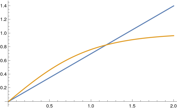
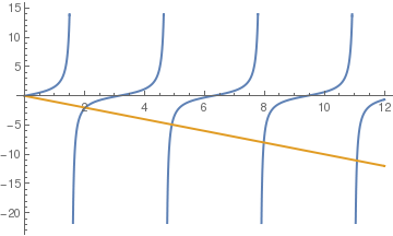
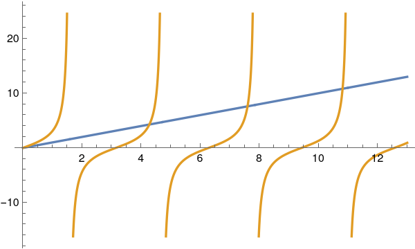
       Graphs of tangent function and the linear function.            Mathematica code

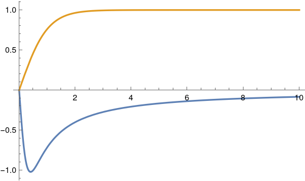
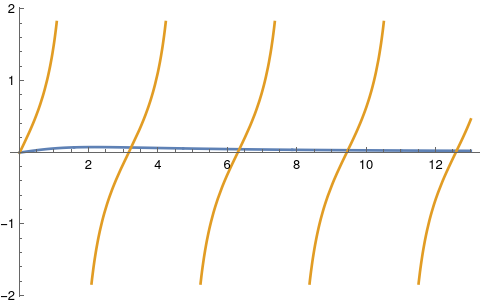
From this figure, we see that the Sturm--Liouville problem has no solutions for λ < 0 when H is positive. However, when H is negative and less than 1, there exists one negative eigenvalue (see figure below).
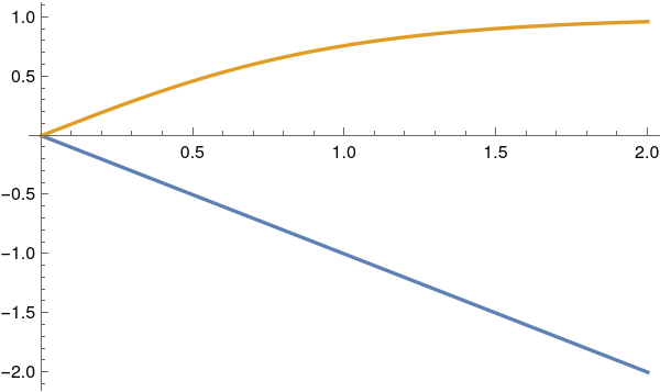
      We plot two functions, 0.7 μ and tangent hyperbolic:
Plot[{0.7*x, Tanh[x]}, {x, 0, 2}, PlotStyle -> Thick]
       Graphs of tangent function and the linear function for H = −0.7.            Mathematica code

When H is negative and its absolute value exceeds 1, the SL-problem has no negative eigenvalues.

Assuming λ = 0, we find the general solution to be a linear function y = cx, with some constant c. From the boundary condition at x = 1, we get

\[ c \left( 1 + H \right) = 0 \qquad \Longrightarrow \qquad H = -1. \]
So we conclude that if H ≠ −1, the SL-problem has no solution when λ = 0.

Assuming λ = ω² is positive, the general solution of the given differential equation becomes

\[ y(x) = c_1 \cos \left( \omega x \right) + c_2 \sin \left( \omega x \right) . \]
From the boundary condition y(0) = 0, it follows that c1 = 0. The boundary condition at x = 1 is satisfied if
\[ c_2 \sin \left( \sqrt{\lambda} \right) + c_2 H \sqrt{\lambda}\,\cos \left( \sqrt{\lambda} \right) =0. \]
Choosing c2 ≠ 0, we see that the last equation is equivalent to
\[ \tan \sqrt{\lambda} = - H \sqrt{\lambda} \qquad \mbox{or} \qquad \tan \mu = -H\,\mu . \tag{3T.3} \]
Let ωn (n = 1, 2, 3, …) be the sequence of positive roots of the transcendent equation (3T.3). Then the eigenvalues and corresponding eigenfunctions are
\[ \lambda_n = \omega_n^2 , \qquad \phi_n (x) = \sin \left( \omega_n x \right) , \qquad n=1,2,3,\ldots . \tag{3T.4} \]

The transcendent equation (3T.3) could be solved only by a numerical solver using, for instance, Newton's method. Nevertheless, if we let \( t = \sqrt{\lambda} , \) then we see from their graphs that there exists an infinite number of roots of \( \tan t = -t . \)

Plot[{Tan[t], -t}, {t, 0, 12}, PlotStyle -> Thick]
Since tangent function has vertical asymptotes at \( t = \frac{\pi}{2} + n\pi , \quad n=0,1,2,\ldots ; \) the roots tn of the equation \( \tan t = -t \) approach
\[ t_n \,\to \frac{\pi}{2} + n\pi \qquad \Longrightarrow \qquad \lambda_n = \left( \frac{\pi}{2} + n\pi \right)^2 \qquad\mbox{as} \quad n \to \infty . \]
The corresponding eigenfunctions (up to arbitrary multiple) are
\[ \phi_n (x) = \sin \left( \sqrt{\lambda_n} x\right) \to \sin \left( \frac{\pi \left( 1 + 2n \right) x}{2} \right) \qquad\mbox{as} \quad n \to \infty . \]
Note that this asymptotic formula is valid only for positive H. For negative H, the SL problem has a sequence of positive eigenvalues, but with different asymptotic behavior.

The principal eigenvalue is λ1 ≈ 2.02876, which we find with the aid of Mathematica:

FindRoot[Tan[k] == -k, {k, 1.6}]
{k -> 2.02876}

Upon setting H = 1, we choose a trial function that satisfies the boundary boundary conditions and calculate the corresponding Rayleigh quotient

\[ R[u] = \frac{\langle u, L\,u \rangle}{\langle u, u \rangle} = \frac{35}{12} \approx 2.91667 \qquad \mbox{for}\quad u(x) = x \left( 2x-3 \right) , \]
with
\[ F[u] = \langle u, L\,u \rangle = \int_0^1 \left( 4x-3\right)^2 {\text d}x = \frac{7}{3} \qquad \langle u, u \rangle = \int_0^1 x^2 (2x-3)^2 {\text d}x = \frac{4}{5} . \]
u[x_] = x*(2*x - 3);
D[x*(2*x - 3), x]
Integrate[(4*x - 3)^2, {x, 0, 1}]
7/3
Integrate[x^2 *(2*x - 3)^2, {x, 0, 1}]
4/5
   ■

Example 3A (third kind boundary conditions): We consider another Sturm--Liouville problem

\[ y'' + \lambda \,y =0 , \qquad y(0) - h\,y'(0) = 0 , \quad y(1) +H\,y'(1 ) =0 . \tag{3A.1} \]
where h and H are some constants. In applications, these constant are usually positive numbers.

As usual, we start analyzing this SL problem with the case when λ = −μ² is negative. The general solution of the differential equation \( y'' - \mu^2 y =0 \) is a linear combination of hyperbolic functions:

\[ y(x) = c_1 \cosh (\mu x) + c_2 \sinh (\mu x) . \tag{3A.2} \]
Substituting this function into boundary conditions, we obtain the system of equations
\[ \begin{split} c_1 - h\,\mu\,c_2 &=0, \\ c_1 \cosh (\mu ) + c_2 \sinh (\mu ) + H \,\mu \left( c_1 \sinh (\mu ) + c_2 \cosh (\mu ) \right) &= 0. \end{split} \tag{3A.3} \]
The corresponding matrix is
\[ {\bf M} = \begin{bmatrix} 1 & -h\,\mu \\ \cosh (\mu ) + H \,\mu \sinh (\mu ) & \sinh (\mu ) + H \,\mu\,\cosh (\mu ) \end{bmatrix} \qquad \Longrightarrow \qquad \det{\bf M} = \sinh (\mu ) + H \,\mu\,\cosh (\mu ) + h\,\mu \left( \cosh (\mu ) + H \,\mu \sinh (\mu ) \right) . \]
The determinant can be simplified as
\[ \det{\bf M} = \left( 1 + hH\,\mu^2 \right) \sinh (\mu ) + \mu \left( h + H \right) \cosh (\mu ) . \]
System of linear equations (3A.3} has a nontrivial solution only when the determinant of M is zero:
\[ \tanh (\mu ) = \frac{\sinh (\mu )}{\cosh (\mu )} = - \frac{\mu \left( h + H \right)}{1 + hH\,\mu^2} . \tag{3A.4} \]
      Upon choosing positive constant h and H to be 2 and 3, respectively, we plot functions in Eq.(3A.4):
Plot[{-5*x/(1 + 6*x*x), Tanh[x]}, {x, 0, 10}, PlotStyle -> Thick]
       Graphs of tangent hyperbolic and the linear function for H = −0.7.            Mathematica code

As it is seen from the figure, the determinant is not zero for any positive values of parameters h and H. Therefore, the eigenvalue of the given problem cannot be negative. Of course, if at leas on of the parameters h or H is negative, it is possible that one eigenvalue is negative.

Let us consider the case when λ = 0. Substituting the general solution y = c₁ + cx into the boundary conditions, we obtain

\[ c_1 - h c_2 =0, \qquad c_1 + c_2 + H c_2 = 0 \qquad \Longrightarrow \qquad c_2 \left( 1 + h + H \right) = 0. \]
Therefore, we conclude that λ = 0 is not an eigenvalue for positive h and H.

Finally, we consider the case of positive eigenvalues: λ = ω² > 0. The general solution of the corresponding differential equation \( y'' + \omega^2 y =0 \) is a linear combination of trigonometric functions:

\[ y(x) = c_1 \cos (\omega x) + c_2 \sin (\omega x) . \tag{3A.5} \]
Substitution of (3A.5) into boundary conditions yields
\[ \begin{split} c_1 - h\,\mu\,c_2 &=0, \\ c_1 \cos (\omega ) + c_2 \sin (\omega ) + H \,\omega \left( -c_1 \sin (\omega ) + c_2 \cos (\omega ) \right) &= 0. \end{split} \tag{3A.6} \]
y[x_] = c1*Cos[m*x] + c2*Sin[m*x];
y[0] - h*D[y[x], x] /. x -> 0
c1 - c2 h m
y[1] + H*D[y[x], x] /. x -> 1
c1 Cos[m] + c2 Sin[m] + H (c2 m Cos[m] - c1 m Sin[m])
This linear system of equations with respect to c₁ and c₂ has a nontrivial solution iff the determinant of the corresponding matrix is zero:
\[ \left( 1 - hH\,\omega^2 \right) \sin\omega + \omega \left( h + H \right) \cos\omega = 0 , \]
M = {{1, -h*m}, {Cos[m] - H*m*Sin[m], Sin[m] + H*m*Cos[m]}};
Det[M]
h m Cos[m] + H m Cos[m] + Sin[m] - h H m^2 Sin[m]
which we rewrite as
\[ \tan \omega = \frac{\sin\omega}{\cos\omega} = - \frac{\omega \left( h + H \right)}{1 - hH\,\omega^2} . \tag{3A.7} \]
      Upon choosing positive constant h and H to be 2 and 3, respectively, we plot functions in Eq.(3A.4):
Plot[-{5*x/(1 - 6*x*x), Tan[x]}, {x, 0, 13}, PlotStyle -> Thick]
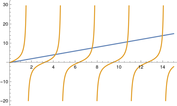
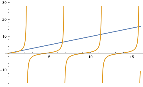
       Graphs of tangent and the rational function for h = 2, H = 3.            Mathematica code

The principal eigenvalue is λ1 ≈ 3.19291, which we find with the aid of Mathematica:
FindRoot[Tan[k] == k/(1 + 6*k^2), {k, 3}]
{k -> 3.19291}
   ■
Theorem 2: Let u and v be linearly independent solutions of regular Sturm--Liouville problem \eqref{EqSturm.5} for the same value of λ. Then λ is an eigenvalue of the Sturm-Liouville problem \eqref{EqSturm.5} if and only if
\begin{equation} \label{EqSturm.6} \det \begin{bmatrix} B_1 [u] & B_a [v] \\ B_b [u] & B_b [v] \end{bmatrix} = 0 . \end{equation}
Let w be a linear combination of these two functions:
\[ w = c_1 u(x) + c_2 v(x) . \]
Function w(x) is a solution of the differential equation \( L \left[ x, \texttt{D} \right] w = \lambda\,w(x) \) for Sturm--Liouville operator L of \eqref{EqSturm.3}. This function satisfies the homogeneous boundary condition if and only if
\[ \begin{bmatrix} B_a [w] \\ B_b [w] \end{bmatrix} = \begin{bmatrix} c_1 B_a [u] + c_2 B_b [v] \\ c_1 B_b [u] + c_2 B_b [v] \end{bmatrix} = \begin{bmatrix} B_a [u] & B_a [v] \\ B_b [u] & B_b [v] \end{bmatrix} \, \begin{bmatrix} c_1 \\ c_2 \end{bmatrix} = \begin{bmatrix} 0 \\ 0 end{bmatrix} . \]
This system of linear equations has a nontrivial solution if and only if \eqref{EqSturm.6} is satisfied.

Example 4: We reconsider differential operators in the first two examples. So we start with the constant coefficient differential operator

\[ L\left[ \texttt{D} \right] = \texttt{D}^2 + 5\,\texttt{D} + 4\,\texttt{I} , \qquad \texttt{D} = \frac{\text d}{{\text d}x} , \quad \texttt{I} = \texttt{D}^0 . \tag{4.1} \]
Upon choosing mixed boundary conditions, the corresponding Sturm--Liouville problem for this differential operator reads as
\[ y'' + 5\,y' + 4\,y + \lambda\,y =0 \quad (0 < x < 1), \qquad y(0) =0, \quad y' (1) = 0. \tag{4.2} \]
Here we use the more compact prime notation (due to Lagrange) for derivatives. To solve this two-point boundary value problem (4.2), we first find the general solution to the differential equation \( y'' + 5\,y' + 4\,y + \lambda\,y =0 . \) The characteristic equation (4.2) is
\[ r^2 + 5\,r + 4 + \lambda = 0 , \]
with zeroes
\[ r_1 = \frac{-5 + \sqrt{25 - 16\lambda}}{2} \qquad\mbox{and} \qquad r_2 = \frac{-5 - \sqrt{25 - 16\lambda}}{2} \]
If λ < 25/16, then r₁ and r₂ are real and distinct, so the general solution of the differential equation (4.2) becomes
\[ y = c_1 e^{r_1 x} + c_2 e^{r_2 x} , \tag{4.3} \]
with some arbitrary constants c₁ and c₂. The boundary conditions require that
\begin{align*} c_1 + c_2 &= 0, \\ c_1 r_1 e^{r_1} + c_2 r_2 e^{r_2} &=0 . \end{align*}
Since the determinant of this system is \( r_2 e^{r_2} - r_1 e^{r_1} \ne 0 , \) the system has only the trivial solution. Therefore λ isn’t an eigenvalue of Eq.(4.2)

If λ = 25/16, then the characteristic equation has a double root r₁ = r₂ = −5/2. Hence, the general solution becomes

\[ y = \left( c_1 + c_2 x \right) e^{-5 x/2} . \tag{4.4} \]
The boundary condition at x = 0 dictates that c₁ = 0. The boundary condition at x = 1 specifies c₂ = 0. Therefore, λ = 25/16 = 1.5625 is not an eigenvalue.

If λ > 25/16 = 1.5625, then

\[ r_1 = -\frac{5}{2} + {\bf j} \omega , \qquad r_2 = -\frac{5}{2} - {\bf j} \omega \qquad ({\bf j}^2 = -1) \]
with
\[ \omega = \sqrt{4\lambda - \frac{25}{4}} \qquad \mbox{or equivalently} \qquad \lambda = \frac{25+4\omega^2}{16} . \]
In this case, the general solution of the differential equation becomes
\[ y = e^{-5x/2} \left( c_1 \cos \omega x + c_2 \sin \omega x \right) . \tag{4.5} \]
The boundary condition y(0) = 0 requires c₁ = 0. The boundary condition at another end leads to
\[ y' (1) = e^{-5/2} c_2 \left( \omega \cos \omega - \frac{5}{2}\, \sin \omega \right) = 0 . \]
Therefore, ω must be a root of the transcendent equation
\[ \omega \cos \omega - \frac{5}{2}\, \sin \omega = 0 \qquad \mbox{or} \qquad \omega = \frac{5}{2}\,\tan \omega . \tag{4.6} \]
Plot[{omega, 5*Tan[omega]/2}, {omega, 0, 15}, PlotStyle -> Thick]
      Then we find a few roots of Eq.(3.3).
sol = FindRoot[x - 5*Tan[x]/2 == 0, {x, 4}]
r1 = x /. sol
4.1726}
sol = FindRoot[x - 5*Tan[x]/2 == 0, {x, 7}]
r2 = x /. sol
7.53357}
sol = FindRoot[x - 5*Tan[x]/2 == 0, {x, 10}]
r3 = x /. sol
10.7674
sol = FindRoot[x - 5*Tan[x]/2 == 0, {x, 14}]
r4 = x /. sol
13.96

For large n, we have asymptotic behavior of the roots:
\[ \omega_n \approx \left( n + \frac{1}{2} \right) \pi , \qquad \mbox{as} \quad n \mbox{ approaches infinity}. \tag{4.7} \]
For example,
\[ \omega_5 \approx 17.1339 \qquad \mbox{and} \qquad \left( 5 + \frac{1}{2} \right) \pi \approx 17.2788 . \]
Let ωn (n = 1, 2, 3, …) be positive roots of Eq.(4.6) to which correspond eigenfunctions
\[ y = \phi_n (x) = e^{-5x /2} \sin \left( \omega_n x \right) , \quad \lambda_n = \frac{25 + 4\omega_n^2}{16} , \qquad n=1,2,3,\ldots . \tag{4.8} \]
A first few eigenvalues are
\[ \lambda_1 \approx 5.91514, \quad \lambda_2 \approx 15.7512 , \quad \lambda_3 \approx 30.5469, \quad \lambda_4 \approx 50.2826. \]


Now we apply Rayleigh–Ritz formula to estimate the principal (lowest) eigenvalue:
\[ \lambda \approx \frac{\langle u, L[u] \rangle}{\langle u, u\rangle} = \frac{F[u]}{\| u \|^2}, \]
where u is a trial function that satisfies the given boundary conditions. We start with a trial function u = x(1 −x)². For this function, we have
\[ L[u] = - \left( \texttt{D}^2 + 5 \texttt{D} + 4 \texttt{I} \right) x\left( 1 - x \right)^2 = - 4\,x^3 - 7\,x^2 + 10\,x -1 . \]
Then
\[ F[u] = \langle u, L[u] \rangle = -\int_0^1 x \left( 1-x \right)^2 \left( 1 - 10\,x + 7\,x^2 + 4\,x^3 \right) {\text d} x = \frac{2}{21} . \]
u[x_] = x*(1 - x)^2 ; D[u[x], x, x] + 5*D[u[x], x] + 4*u[x]
1 - 10 x + 7 x^2 + 4 x^3
-Integrate[u[x]*(1 - 10 x + 7 x^2 + 4 x^3), {x, 0, 1}]
2/21
Integrate[u[x]^2 , {x, 0, 1}]
1/105
Therefore,
\[ \lambda \approx \frac{\langle u, L[u] \rangle}{\langle u, u\rangle} = 10. \]
However, suppose we would like to transfer the given differential operator to a self-adjoint normal form. So we make substitution
\[ y = e^{-5x/2} u \qquad \Longrightarrow \qquad y' = e^{-5x/2} \left( u' -\frac{5}{2} \, u \right) , \quad y'' = e^{-5x/2} \left( u'' -5\,u' + \frac{25}{4}\,u \right) . \]
This leads to
\[ \left( \texttt{D}^2 + 5\,\texttt{D} + 4\, \texttt{I} \right) e^{-5x/2} u = e^{-5x/2} \left( u'' - \frac{9}{4}\, u\right) . \]
This yields the following Sturm--Liouville problem for function u:
\[ u'' - \frac{9}{4}\, u + \lambda\,e^{5x/2} u = 0, \qquad u(0) = 0, \quad u' (1) = \frac{5}{2}\,u(1) . \]
To estimate the princioal eigenvalue, we calculate integrals for the trial function \( \displaystyle u(x) = x \left( \cosh (3x/2) + \sinh (3x/2) \right): \)
\begin{align*} F[u] &= \langle u, L[u] \rangle = \frac{9}{4} \int_0^1 u(x)^2 {\text d} x + \int_0^1 \left( u' \right)^2 {\text d} x \approx 36.4902 , \\ \| u \|^2_w &= \int_0^1 u^2 (x) \, e^{5x/2}\,{\text d}x \approx 31.2409 . \end{align*}
u[x_] = x*(Cosh[3/2*x] + Sinh[3*x/2]); Integrate[u[x]*(9*u[x]/4) + (D[u[x], x]^2), {x, 0, 1}]
1/6 (-2 + 11 E^3)
Integrate[u[x]*u[x]*Exp[5*x/2], {x,0,1}]
(2 (-8 + 85 E^(11/2)))/1331
This provides approximation to the principal eigenvalue to be
\[ \frac{F[u]}{\| u \|^2} \approx 1.16802 \]
   ■

Example 4D: We consider the Sturm--Liouville problem

\[ y'' - 4\,y' + 4\,y + \lambda\, y = 0 , \qquad y' (0) = 0, \qquad y(1) + 3\,y'(1) = 0 , \tag{4D.1} \]
for not self-adjoint operator
\[ L \left[ \texttt{D} \right] = - \left( \texttt{D} -2\texttt{I} \right)^2 = - \left[ \texttt{D}^2 - 4\,\texttt{D} + 4\,\texttt{I} \right] . \]
The general solution of ODE from Eq.(4D.1) depends on the roots of the characteristic equation
\[ r^2 - 4\,r + 4 + \lambda = 0 \qquad \Longrightarrow \qquad r_{1,2} = 2 \pm \sqrt{- \lambda} . \tag{4D.2} \]

If λ = −μ² < 0, then quadratic equation (4D.2) has two distinct real roots, and the general solution of Eq.(4D.1) can be written as

\[ y = e^{2 x} \left[ c_1 \cosh (\mu x) + c_2 \sinh (\mu x) \right] . \]
Substitution of this function into the given boundary conditions yields a system of linear equations (according to Theorem 2) with matrix
\[ {\bf M} = \begin{bmatrix} 2 & \mu \\ 7\,\cosh (\mu ) + 3\mu\, \sinh (mu ) & 7\,\sinh (\mu ) + 3 \mu\, \cosh (\mu )\end{bmatrix} . \]
Its determinant is
M = {{2, m}, {3 m Sinh[m] + 7 Cosh[m], 3 m Cosh[m] + 7 Sinh[m]}};
Det[M]
-m Cosh[m] + 14 Sinh[m] - 3 m^2 Sinh[m]
\[ \det {\bf M} = \left( 14 - 3\mu^2 \right) \sinh (\mu ) - \mu\,\cosh (\mu ) . \tag{4D.3} \]
      Upon plotting the determinant, we see that it has one real root μ = 1.9942. Therefore, this Sturm--Liouville problem has one negative eigenvalue λ = −μ² = −3.97683.
FindRoot[-m Cosh[m] + 14 Sinh[m] - 3 m^2 Sinh[m] == 0, {m, 2}]
{m -> 1.9942}
Plot[-m Cosh[m] + 14 Sinh[m] - 3 m^2 Sinh[m], {m, 0, 2.5}, PlotStyle -> Thick]
       Graphs of determinant (4D.3).            Mathematica code

Therefore, the given Sturm--Liouvlle problem has one negative eigenvalue

\[ \lambda = - \mu^2 = - \left( 1.9942 \right)^2 \approx - 3.97683. \]


The case λ = 0 cannot provide an eigenvalue because function \( \displaystyle y = e^{2x} \left( 1 - 2x \right) \) cannot satisfy the boundary condition at x = 1.

Now we consider the case when λ = ω² > 0. The general solution of differential equation \( \displaystyle y'' - 4\,y' + 4\,y + \omega^2 y = 0 \) is

\[ y = e^{2x} \left[ c_1 \cos (\omega x) + c_2 \sin (\omega x) , \right] \qquad \omega^2 = \lambda . \]
The first boundary condition
\[ y' (0) = 2\,c_1 + \omega\,c_2 \]
dictates 2c₁ = −ω c₂. Therefore, the general solution is proportional to
\[ y = e^{2x} \left[ -\omega\, \cos (\omega x) + 2\, \sin (\omega x) , \right] , \qquad \omega^2 = \lambda . \]

Substituting \( \displaystyle y = e^{2x} \left[ 2\,\sin (\omega x) - \omega\,\cos (\omega x) \right] \) into the boundary condition at x = 1, we obtain

y[x_] = Exp[2*x]*(2*Sin[m*x] - m*Cos[m*x])
y[1] + 3*D[y[x], x] /. x -> 1
Simplify[%]
E^2 (-m Cos[m] + (14 + 3 m^2) Sin[m])
\[ y(1) + 3y' (1) = e^{2} \left[ -\omega\,\cos\omega + \left( 14 + 3\,\omega^2 \right) \sin\omega \right] = 0. \tag{4D.4} \]
Upon dropping the exponential term e², Eq.(4D.4) is fulfilled iff ω is a positive root of transcendent equation
\[ \left( 14 + 3\,\omega^2 \right) \sin\omega = \omega\,\cos\omega \qquad \iff \qquad \tan\omega = \frac{\omega}{14 + 3\,\omega^2} . \tag{4D.5} \]
      Upon plotting two functions, r/(14 + 3r²) and tan(r), we see that they meet at discrete number of points. Hence, λ > 0 provides an eigenvalue.
Plot[{x/(14 + 3 x^2), Tan[x]}, {x, 0, 13}, PlotStyle -> Thick]
       Graphs of cotangent and the linear function for −ω.            Mathematica code

Let ωn be the sequence of of roots of transcendent equation (4D.5), then eigenvalues and eigenfunctions are expressed through these roots
\[ \lambda_n = \omega_n^2 , \qquad \phi_n (x) = e^{2x} \left[ 2\,\sin (\omega_n x) - \omega_n \cos (\omega_n x) \right] , \qquad n=1,2,3,\ldots . \tag{4D.6} \]
The lowest positive eigenvalue is
\[ \lambda_1 = \omega_1^2 \approx 10.3229 , \qquad \mbox{with} \quad \omega_1 \approx 3.21292. \]
sol = FindRoot[(14 + 3*m^2)*Sin[m] == m*Cos[m], {m, 3}];
omega1 = m/. sol;
lambda1 = omega1^2
10.3229
The next to lowest positive eigenvalue is 40.0729 as Mathematica confirms:
sol2 = FindRoot[(14 + 3*m^2)*Sin[m] == m*Cos[m], {m, 6}];
omega2 = m/. sol2;
lambda2 = omega2^2
40.0729
We choose a trial function that satisfies the boundary conditions and calculate the corresponding Rayleigh quotient
\[ R[u] = \frac{\langle u, L\,u \rangle}{\langle u, u \rangle} = 8 \qquad \mbox{for}\quad u(x) = x^2 \left( 1 - 2\,x + x^2 \right) , \]
with
\[ \langle u, L\,u \rangle = -\int_0^1 x^2 (x-1)^2 \left( 2 - 20 x + 40 x^2 - 24 x^3 + 4 x^4 \right) {\text d}x = \frac{4}{315} \qquad \langle u, u \rangle = \int_0^1 x^4 (x-1)^2 {\text d}x = \frac{1}{630} . \]
u[x_] = x^2 *(x - 1)^2; Integrate[-u[x]*(D[u[x], x, x] - 4*D[u[x], x] + 4*u[x]), {x, 0, 1}]
4/315
Integrate[x^4*(x - 1)^4, {x, 0, 1}]
1/630
Therefore, we see that the Rayleigh--Ritz formula does not work in this example because the operator L is not self-adjoint. So we transfer the differential equation (4D.1) into normal form by substitution:
\[ y = e^{2x} u \qquad \Longrightarrow \qquad y' = e^{2x} \left( 2\,u + u' \right) , \quad y'' = e^{2x} \left( 4\,u + 4\,u' + u'' \right) . \]
This yields the Sturm--Liouville problem for function u(x):
\[ u'' + e^{-2x} \lambda \, u = 0, \qquad 2\,u(0) + u' (0) =0, \quad 7\,u(1) + 3\,u' (1) = 1. \tag{4D.7} \]
A trial function u(x) = (1 −x)² satisfies the boundary conditions in SL-problem (4D.7), so we use this function to estimate the Rayleigh quotient:
\[ R[u] = \frac{F[u]}{\| u \|^2_w} \approx 8.97876, \qquad F[u] = \int_0^1 \left( u' \right)^2 {\text d}x = \frac{4}{3} , \quad \| u \|^2_w = \int_0^1 u^2 e^{-2x} {\text d}x \approx 0.148499. \]
u[x_] = (x - 1)^2;
Integrate[(D[u[x], x])^2 , {x, 0, 1}]
4/3
Integrate[Exp[-2*x]*(u[x])^2 , {x, 0, 1}]
1/4 - 3/(4 E^2)
   ■

Example 4C: We consider the Sturm--Liouville problem

\[ y'' - 4\,y' + 13\,y + \lambda\, y = 0 , \qquad y' (0) = 0, \qquad y(1) = 0 , \tag{4C.1} \]
for not self-adjoint operator
\[ L \left[ \texttt{D} \right] = - \left( \texttt{D} -2\texttt{I} \right)^2 - 9\,\texttt{I} = - \left[ \texttt{D}^2 - 4\,\texttt{D} + 13\,\texttt{I} \right] . \]
The general solution of differential equation (4C.1) depends on the roots of the characteristic equation
\[ (r -2)^2 + 9 + \lambda = 0 \qquad \Longrightarrow \qquad r_{1,2} = 2 \pm \sqrt{-9-\lambda} . \tag{4C.2} \]
If λ < −9, the quadratic equation (4C.2) has two distinct real roots, and the general solution of Eq.(4C.1) becomes
\[ y = e^{2x} \left[ c_1 \cosh (\omega\,x) + c_2 \sinh (\omega\,x) \right] , \qquad \omega = \sqrt{-9-\lambda} > 0. \tag{4C.3} \]
To satisfy the boundary condition at x = 0, we have to fulfill the condition
\[ y' (0) = 2\,c_1 + c_2 \omega = 0. \]
The boundary condition at another end = 1 dictates
\[ y (1) = e^2 \left[ c_1 \cosh \omega + c_2 \sinh\omega \right] = 0. \]
Therefore, ω has to satisfy the transcendent equation
\[ -\omega\,\cosh\omega + 2\,\sinh\omega = 0 \qquad\Longrightarrow \qquad \tanh \omega = \frac{\omega}{2} , \]
which has no real root. Hence, we conclude that λ < −9 cannot provide a nontrivial solution.

If λ = −9, then the differential equation has the general solution (with two arbitrary constants c₁ and c₂)

\[ y = e^{2x} \left( c_1 + c_2 x \right) . \]
This function cannot satisfy two boundary conditions in Eq.(4C.1); therefore, we dismiss this case for providing an eigenvalue.

Now let λ > −9. Then the differential equation \( \displaystyle y'' - 4\,y' + 13\,y + \lambda\, y = 0 \) has the general solution:

\[ y = e^{2x} \left[ c_1 \cos (\omega\,x) + c_2 \sin (\omega\,x) \right] , \qquad \omega = \sqrt{9+\lambda} . \tag{4C.4} \]
Substituting this function (4C.4) into boundary condition, we obtain
\[ \omega\,\cos\omega = 2\,\sin\omega \qquad\Longrightarrow \qquad \omega = 2\,\tan\omega . \tag{4C.5} \]
      Upon plotting two functions, x and 2tan(x), we see that they have infinite many discrete roots. Hence λ > −9 provides an eigenvalue.
Plot[{x, 2*Tan[x]}, {x, 0, 13}, PlotStyle -> Thick]
       Graphs of tangent and the linear function for positive ω.            Mathematica code

Let ωn denote the n-th root of transcendent equation (4C.5), then eigenvalues and eigenfunctions are expressed through these roots:
\[ \lambda_n = \omega_n^2 -9 , \qquad \phi_n (x) = e^{2x} \left[ 2\,\sin (\omega_n x) - \omega_n \cos (\omega_n x) \right] , \qquad n=1,2,3,\ldots . \tag{4C.6} \]
The corresponding principal eigenvalue is 9.27376 as Mathematica confirms:
sol = FindRoot[2*Tan[x] == x, {x, 4}];
omega1 = x /. sol;
lambda1 = omega1^2 - 9
9.27376
We choose a function that satisfies the mixed boundary conditions and calculate the corresponding Rayleigh quotient
\[ R[u] = \frac{\langle u, L\,u \rangle}{\langle u, u \rangle} = 1 \qquad \mbox{for}\quad u(x) = x^2 \left( x-1 \right) , \]
with
\[ \langle u, L\,u \rangle = \int_0^1 x^2 (x-1) \left( 2 - 14 x + 25 x^2 - 13 x^3 \right) {\text d}x = \frac{1}{105} \qquad \langle u, u \rangle = \int_0^1 x^4 (x-1)^2 {\text d}x = \frac{1}{105} . \]
u[x_] = x* x*(x - 1); Integrate[-u[x]*(D[u[x], x, x] - 4*D[u[x], x] + 13*u[x]), {x, 0, 1}]
1/105
Integrate[x^4*(x - 1)^2, {x, 0, 1}]
1/105


Integrating factor: μ(x)

Multiplying the given differential equation (4C.1) by the integrating factor, we reduce it to the following form:
\[ \frac{\text d}{{\text d}x} \left( e^{-4x} \frac{{\text d}y}{{\text d}x} \right) + 13\, e^{-4x} y + \lambda\,e^{-4x} y = 0 . \qquad y' (0) = 0, \quad y(1) = 0. \tag{4C.7} \]
This is classical Sturm--Liouville problem \eqref{EqSturm.1}, \eqref{EqSturm.2}, with \( p(x) = e^{-4x} \) \( q(x) = -13\,e^{-4x} \) and weight function w(x) = p(x) > 0.

The Sturm--Liouville problem (4C.7) has exactly the same solution as was obtained previously because multiplication by a function μ(x) ≠ 0 does not change its solution. However, calculation of Rayleigh quotient will be different because the inner product should incorporate the weight function:

\[ \langle u, L\,u \rangle = \int_0^1 e^{-4x} x^2 (x-1) \left( 2 - 14 x + 25 x^2 - 13 x^3 \right) {\text d}x = \frac{3417 e^{-4} - 61}{1024} \qquad \langle u, u \rangle = \int_0^1 x^4 (x-1)^2 e^{-4x} {\text d}x = \frac{9-437 e^{-4}}{1024} , \]
and
\[ \langle u, u \rangle = \int_0^1 x^4 (x-1)^2 e^{-4x} {\text d}x = \frac{9- 437\,e^{-4}}{1024} \approx 0.000972721. \]
u[x_] = x* x*(x - 1); Integrate[-Exp[-4*x]*u[x]*(D[u[x], x, x] - 4*D[u[x], x] + 13*u[x]), {x, 0, 1}]
(-61 + 3417/E^4)/1024
Integrate[Exp[-4*x]*x^4*(x - 1)^2, {x, 0, 1}]
(9 - 437/E^4)/1024
The corresponding Rayleigh quotient becomes
\[ R[u] = \frac{\langle u, L\,u \rangle}{\langle u, u \rangle} = 1.5908 \qquad \mbox{for}\quad u(x) = x^2 \left( x-1 \right) , \]
((-12585 + E^8)/(131072 E^8))/((9 - 437/E^4)/1024)
(-12585 + E^8)/(128 (9 - 437/E^4) E^8)
N[%]
-0.0252697


Transfering to self-adjoint normal form:

WE make substitution:
\[ y = e^{2x} u \qquad \Longrightarrow \qquad y' = e^{2x} \left( 2\,u + u' \right) , \quad y'' = e^{2x} \left( 4\,u + 4\,u' + u'' \right) . \]
This yields the Sturm--Liouville problem for function u(x):
\[ u'' + 9\, u + e^{-2x} \lambda \, u = 0, \qquad 2\,u(0) + u' (0) =0, \quad u(1) = 1. \tag{4D.7} \]
We choose a trial function u(x) = (1 −x)² that satisfies the boundary conditions in Eq.(4D.7). Then
\begin{align*} F[u] &= \int_0^1 \left( u' \right)^2 {\text d} x -9 \int_0^1 \left( u \right)^2 {\text d}x = - \frac{7}{15} \approx -0.466667, \\ \| u \|^2_w &= \int_0^1 u^2 (x)\, e^{-2x} {\text d} x \approx 0.148499. \end{align*}
u[x_] = 1 - 2*x + x^2 ;
Integrate[(D[u[x], x])^2 , {x, 0, 1}] - 9* Integrate[(u[x])^2 , {x, 0, 1}]
-(7/15)
N[%]
-0.466667
Integrate[(u[x])^2 * Exp[-2*x], {x, 0, 1}]
1/4 - 3/(4 E^2)
N[%]
0.148499
So the Rayleigh quotient gives an approximation to the lowest eigenvalue as
\[ \lambda_0 \approx -3.14256 . \]
   ■

Properties of Eigenvalues and Eigenfuncnctions


Many properties of solutions are based on the following identity.
Lagrange identity: For any two twice continuously differentiable on a closed interval [𝑎, b] functions u(x) and v(x), the following identity holds
\[ v\,L\left[ x, \texttt{D} \right] u - u\,L\left[ x, \texttt{D} \right] v = \frac{\text d}{{\text d}x} \left[ p(x) \left( v\, \frac{{\text d}u}{{\text d}x} - u \,\frac{{\text d}v}{{\text d}x}\right) \right] , \]
where L is the self-adjoint differential operator \eqref{EqSturm.3}.

The Lagrange identity is established by integration by parts and is left to the reader.

Let \( \displaystyle L\left[ x, \texttt{D} \right] = q(x)\,\texttt{I} - \texttt{D}\,p(x)\,\texttt{D} \) be the Sturm--Liouville differential operator from \eqref{EqSturm.3}. The expression
\begin{equation} \label{EqSturm.8} R[u] = \frac{\langle u, L\,u \rangle}{\langle u , u \rangle_w} = \dfrac{p(x) \left( v\, \frac{{\text d}u}{{\text d}x} - u \,\frac{{\text d}v}{{\text d}x}\right)_{x=a}^{x=b} + \int_a^b \left[ p \left( u' \right)^2 + q \left( u \right)^2 \right] {\text d}x}{\int_a^b \left( u \right)^2 w(x)\,{\text d}x} \end{equation}
is called the Rayleigh quotient. If u is a solution of the regular Sturm--Liouville problem \eqref{EqSturm.1}, \eqref{EqSturm.2}. then the Rayleigh quotient is positive when p(x) > 0, q(x) ≥ 0.

The Rayleigh quotient is named in honour of John William Strutt, Lord Rayleigh (1842-1919), who made a great number of contributions to the study of sound and wave phenomena in general. He was awarded the 1904 Nobel Prize in Physics for the discovery of argon. He also developed a number of important approximation methods that have become fundamental tools in applied mathematics and physics. Presented below the Rayleigh--Ritz formula is one of them.

The principal eigenvalue, also known as the ground state energy, of a Sturm-Liouville problem is the minimal eigenvalue λ0. The principal eigenfunction is the eigenfunction corresponding to the principal eigenvalue.

The following functional is associated with the Sturm-Liouville operator \eqref{EqSturm.3}

\[ F[u] = \int_a^b \left[ p(x)\left( u' \right)^2 + q(x)\,u^2 (x) \right] {\text d} x , \]
whose corresponding Euler--Lagrange equation is given by the Sturm-Liouville equation. A minimizer will yield the equation \( \displaystyle F'[u] = \lambda\,u , \) assuming that p(x) ≥ α > 0, q(x) ≥ 0. The functional F[u] appears in the numerator of the Rayleigh quotient \eqref{EqSturm.8} and it is related to the eigenvalues of classical Sturm--Liouville problem. Indeed, consider equation \eqref{EqSturm.1}, written for any twice differentiable function u(x):
\[ \frac{\text d}{{\text d}x} \left[ p(x)\,\frac{{\text d}u}{{\text d}x} \right] - q(x)\, u + \lambda \,w (x)\,u(x) =0 , \qquad a < x < b . \]
Multiplying this equation by u(x) and integrating, we obtain
\[ \int_a^b u(x)\,\frac{\text d}{{\text d}x} \left[ p(x)\,\frac{{\text d}u}{{\text d}x} \right] \,{\text d}x - \int_a^b q(x)\, u^2 {\text d}x + \lambda \,\int_a^b w (x)\,u^2 (x)\,{\text d}x =0 . \]
Integrating by parts in the first term, we get (assuming that u(x) in addition satisfies the boundary conditions \eqref{EqSturm.2})
\[ -\int_a^b \left[ p \left( u' \right)^2 + q\left( u \right)^2 \right] {\text d}x + \lambda \,\int_a^b w (x)\,u^2 (x)\,{\text d}x =0 . \]
Integrating by parts in the first term, we get (assuming that u(x) in addition satisfies the boundary conditions \eqref{EqSturm.2})
\[ -\int_a^b \left[ p \left( u' \right)^2 + q\left( u \right)^2 \right] {\text d}x + \lambda \,\int_a^b w (x)\,u^2 (x)\,{\text d}x =0 . \]
Any function having square integrable derivative (du/dx ∈ 𝔏²) and satisfying the boundary conditions \eqref{EqSturm.2} is called a trial function for the given Sturm--Liouville problem \eqref{EqSturm.5}. Actually, all eigenvalues are extrema of the Rayleigh quotient. So higher eigenvalues can be evaluated by a process called deflation algorithm (sequential elimination of first determined eigenfunctions from the domain).
Theorem 3: The principal eigenvalue λ0 of a regular Sturm-Liouville problem \eqref{EqSturm.1}, \eqref{EqSturm.2} satisfies the variational principle, known as the Rayleigh-Ritz formula:
\[ \lambda_0 = \inf_{u\in D, \ u\ne 0} R[u] , \]
where D = D(L) is the domain of the Sturm-Liouville operator \eqref{EqSturm.3} in the Hilbert space 𝔏² (this means that u is twice continuously differentiable functions on [𝑎, b] that satisfy the corresponding boundary conditions).

Note that Theorem 3 is valid for trial functions that have only first integrable derivative---having second derivative is not needed for formula \eqref{EqSturm.8}.

Proof of this statement is a subject of the “Calculus of Variations,” and it relies on some facts that were established by mathematicians:
  • The domain of the Sturm--Liouville operator is dense in the Hilbert space 𝔏².
  • The set of the eigenfunctions possess orthonormality property and is complete in the domain of the SL operator.
  • The eigenvalues of a SL problem are bounded from below.
  • The eigenfunction expansion of a twice continuously differentiable function converges uniformly on [𝑎, b].
For u from the domain of the SL operator, we have
\begin{align*} \langle u, L\,u \rangle &= \left\langle \sum_{n\ge 0} c_n \phi_ (x), L \left[ x, \texttt{D} \right] \sum_{n\ge 0} c_n \phi_ (x) \right\rangle = \left\langle \sum_{n\ge 0} c_n \phi_ (x), \sum_{n\ge 0} c_n L \left[ x, \texttt{D} \right] \phi_ (x) \right\rangle \end{align*}
because every function u from the domain of the SL operator can be expanded into a uniformly convergent series with respect to the set of eigenfunctions. Since each function ϕn is an eigenfunction, we have
\begin{align*} \langle u, L\,u \rangle &= \left\langle \sum_{n\ge 0} c_n \phi_ (x), \sum_{n\ge 0} c_n \lambda_n \phi_ (x) \right\rangle \\ &= \sum_{k\ge 0} \sum_{n\ge 0} \left\langle c_k \phi_k (x) , \lambda_n c_n \phi_n (x)\right\rangle \\ &= \sum_{k\ge 0} \sum_{n\ge 0} c_k^{\ast} c_n \lambda_n \left\langle \phi_k (x) , \phi_n (x)\right\rangle \\ &= \sum_{n\ge 0} \left\vert c_n \right\vert^2 \lambda_n \ge \lambda_0 \sum_{n\ge 0} \left\vert c_n \right\vert^2 \\ & \ge \lambda_0 \| u \|^2 \end{align*}
because
\[ \| u \|^2 = \langle u, u \rangle = \sum_{n\ge 0} c_n^2 , \]
which Parseval's identity (it is equivalent to completeness of the set of eigenfunctions).

Theorem 4: Properties of the regular Sturm--Liouville problem \eqref{EqSturm.1}, \eqref{EqSturm.2}.
Suppose that functions p(x), p'(x), q(x), ρ(x) are continuous on [𝑎, b], and also p(x) and ρ(x) are positive. Then the Sturm–Liouville problem \eqref{EqSturm.5} has the following properties.
  1. There exists an infinite number of real eigenvalues that can be arranged in increasing order λ1 < λ2 < λ3 < … λn < … such that λn →∞ as n→∞.
  2. For each eigenvalue there is only one linearly independent eigenfunction (up until nonzero multiple). In other words, all eigenvalues are simple.
  3. Eigenfunctions corresponding to different eigenvalues are linearly independent.
  4. The set of eigenfunctions { ϕn } corresponding to the set of eigenvalues is orthogonal with respect to the weight function w(x) on the interval x ∈ [𝑎, b]:
    \[ \left\langle \phi_n , \phi_k \right\rangle = \int_0^{\ell} \phi_n (x)^{\ast} \phi_k (x)\,w (x)\,{\text d}x = 0 \qquad \mbox{for} \quad n\ne k. \]
Note: In Sturm--Liouville problems that do not involve self-adjoint operators, the eigenvalues and eigenfunctions may have similar properties to those outlined in Theorem 4. However, the theory of such operators is more complicated, so we restrict our attention to Sturm--Liouville operators.
Since the proof of this part requires a solid knowledge of many topics, we just outline the idea to convince the reader that the statement is true.

It is known that the domain D = D(L) of the Sturm-Liouville operator \eqref{EqSturm.3} is dense in the Hilbert space 𝔏². Then the principal eigenvalue λ0 can be determined by the Rayleigh-Ritz formula:

\[ \lambda_0 = \inf_{u\in D, \ u\ne 0} R[u] . \]
We denote by u0 an eigenfunction corresponding to the principal eigenvalue. Then the next eigenvalue λ₁ can be found from the formula
\[ \lambda_1 = \inf_{u\in D, \ u\perp u_0} R[u] . \]
This eigenvalue λ₁ is larger than λ₀ because the infinimum is taken over a smaller space from which one dimensional space spanned on the principal eigenfunction is removed. We denote by u₁ an eigenfunction corresponding to the eigenvalue λ₁ and remove from the domain D of the Sturm--Liouville operator two dimensional subspace spanned on two eigenfunctions, u₀ and u₁. This allows us to evaluate the next eigenvalue:
\[ \lambda_2 = \inf_{u\in D, \ u\perp u_0 \& u\perp u_1} R[u] . \]
Similarly, λ₂ > λ₁ > λ₀ because the infinimum is taken over smaller space in the latter Rayleigh-Ritz formula.

In general, we introduce finite linear spaces

\[ W_n = \mbox{span}[u_0 , u_1 , \ldots u_n ] \qquad\mbox{and their complements} \qquad V_n = W_n^{\perp} \cap D . \]
Hence, we have nesting
\[ V_n = W_n^{\perp} \cap D \subset V_{n-1} \subset V_{n-2} \subset \cdots \subset V_1 \subset V_0 = D . \]
Because of this nesting, every next eigenvalue λn is larger than all previously obtained eigenvalues because it is determined by the Rayleigh-Ritz formula:
\[ \lambda_n = \inf_{u\in D, \ u\in V_n} R[u] . \]
Since the domain D of the Sturm-Liouville operator \eqref{EqSturm.3} is dense in the infinite dimensional Hilbert space 𝔏², the number of eigenvalues is infinitely numerable.
Sturm did not prove by himself the existence of eigenvalues for regular Sturm--Liouville problems---it was done more than 70 years later, at the beginning of twenteen century. Usually proof of part (a) is accomplished by transfering the boundary value problem for unbounded Sturm--Liouville operator into equivalent integral equation that is actually the inverse operator for the Sturm--Liouville operator. The corresponding integral equation defines a bounded compact operator, for which Hilbert-Schmidt theorem is applied.
Let α and β be arbitrary numbers from the closed interval [𝑎, b] where Sturm--Liouville problem \eqref{EqSturm.1}, \eqref{EqSturm.2} is given. Let u(x) and v(x) be two eigenfunctions corresponding to an eigenvalue λ.

Integrating the Lagrange identity over interval {α, β], we obtain

\begin{align*} 0 &= \left\langle L\left[ x, \texttt{D} \right] u , v \right\rangle - \left\langle u , L\left[ x, \texttt{D} \right] v \right\rangle = \int_{\alpha}^{\beta} \frac{\text d}{{\text d}x} \left[ p(x) \left( v\, \frac{{\text d}u}{{\text d}x} - u \,\frac{{\text d}v}{{\text d}x}\right) \right] {\text d} x \\ &= p(\beta ) \left( v\, \frac{{\text d}u}{{\text d}x} - u \,\frac{{\text d}v}{{\text d}x}\right)_{x=\beta} - p(\alpha ) \left( v\, \frac{{\text d}u}{{\text d}x} - u \,\frac{{\text d}v}{{\text d}x}\right)_{x=\\alpha} . \end{align*}
Observing that the expression in parenthesis is just the Wronskian f two functions,
\[ W(x) = v\, \frac{{\text d}u}{{\text d}x} - u \,\frac{{\text d}v}{{\text d}x} , \]
we rewrite the latter identity as
\[ 0 = p(\beta ) \,W(\beta ) - p(\alpha )\,W(\alpha ) \qquad \Longrightarrow \qquad p(x)\,W(x) = \mbox{constant} . \]
Since both functions, u(x) and v(x), satisfy the homogeneous boundary conditions \eqref{EqSturm.2}, we conclude that
\[ p(x )\,W(x) = 0 \qquad \Longrightarrow \qquad W(x) = 0 . \]
Therefore, the Wronskian of two eigenfunctions is zero, so they are linearly dependent.
Let ϕ(x) and ψ(x) be two eigenfunctions corresponding to two distinct eigenvalues λ and μ, respectively. Then using the Lagrange identity, we have
\begin{align*} 0 &= \left\langle L\left[ x, \texttt{D} \right] \phi , \psi \right\rangle - \left\langle \phi , L\left[ x, \texttt{D} \right] \psi \right\rangle \\ &= -\lambda \langle \rho\,\phi , \psi \rangle + \mu \langle \phi, \rho\,\psi \rangle \\ &= \left( \mu - \lambda \right) \int_a^b {\text d} x\,\rho (x)\,\phi (x)^{\ast} \psi (x) . \end{align*}
Since we have assumed that μ ≠ λ, it follows that
\[ \int_a^b {\text d} x\,\rho (x)\,\phi (x)^{\ast} \psi (x) = 0. \]
Let ϕ(x) be an eigenfunction corresponding to eigenvalue λ, and &psi(x) be an eigenfunction corresponding to eigenvalue μ, with μ ≠ λ. Then we have
\[ L \left[ x, \texttt{D} \right] \phi (x) = \lambda\,\rho (x)\,\phi (x) \qquad\mbox{and} \qquad L \left[ x, \texttt{D} \right] \psi (x) = \lambda\,\rho (x)\,\psi (x) . \]
Using Lagrange's identity, we get
\[ \int_a^b \left( \psi\,L \left[ x, \texttt{D} \right] \phi (x) \,\vert \,\phi\, L \left[ x, \texttt{D} \right] \psi (x) \right) {\text d}x = \left[ p(x) \left( \psi\, \frac{{\text d}\phi}{{\text d}x} - \phi \,\frac{{\text d}\psi}{{\text d}x}\right) \right]_{x=1}^{x=b} = 0. \]
On the other hand, we have
\[ \int_a^b \left( \psi\,L \left[ x, \texttt{D} \right] \phi (x) \,\vert \,\phi\, L \left[ x, \texttt{D} \right] \psi (x) \right) {\text d}x = \int_a^b \left( \psi\,\lambda\,\rho\phi - \phi\,\mu \,\rho\,\psi \right) {\text d}x = \left( \lambda - \mu \right) \int_a^b \psi\,\phi\,\rho\,{\text d}x = \left( \lambda - \mu \right) \left\langle \psi , \psi \right\rangle . \]
Since λ ≠ μ, we obtain orthogonality of eigenfunctions ψ and φ.

When zero is an eigenvalue, we usually start labeling the eigenvalues at 0 rather than at 1 for convenience. That is we label the eigenvalues 0 = λ0 < λ1 < λ2 < ···. It is convenient arrangjng eigenvalues in an increasing order because it enables us to arrange the corresponding egenfunctions

\[ y_0 (x), \quad y_1 (x) , \quad y_2 (x) , \quad \cdots \quad y_n (x) , \cdots \]
in their own natural order. Note that the eigenfunctions are not unique---they are determined up to a nonzero constant factor.

Example 5: We reconsider the Euler differential operator from Example 2; now we analyze the corresponding Sturm--Liouville problem:

\[ x^2 y'' + 3x\,y' - 3\,y + \lambda\,y = 0, \qquad y(1) = 0, \quad y' (2) = 0. \tag{5.1} \]
Upon seeking its solution as a power function: y(x) = xr, we obtain the indicial equation
\[ r(r-1) + 3r - 3 + \lambda = 0 \qquad \Longrightarrow \qquad r_{1,2} = -1 \pm \sqrt{1+3-\lambda} . \tag{5.2} \]
Solve[r*(r - 1) + 3*r - 3 + a == 0, r]
{{r -> -1 - Sqrt[4 - a]}, {r -> -1 + Sqrt[4 - a]}}
The general solution of differential equation in (5.1) depends on the value under the radical. Hence, we consider three cases.

If λ < 4, then the indicial equation (5.2) has two real roots, so the general solution of Eq.(5.1) is

\[ y = c_1 x^{-1 + \mu} + c_2 x^{-1-\mu} , \qquad \mu = \sqrt{4 - \lambda} > 0, \]
where c₁ and c₂ are aritrary constants. Substituting this function into mixed oundary conditions, we get
\[ c_1 + c_2 = 0 , \qquad \left( -1+ \mu \right) c_1 2^{\mu -2} - \left( 1+ \mu \right) c_2 2^{-2\mu} =0 , \]
which is reduced to
\[ \left( -1+ \mu \right) 2^{\mu -2} = \left( 1+ \mu \right) 2^{-2\mu} . \]
Since the latter equation has no solution, we dismiss this case for eigenvalues.

If λ = 4, The indicial equation becomes \( \displaystyle r(r+2) + 1 = (r +1)^2 = 0, \) and the general solution of ODE from Eq.(5.1) becomes

\[ y = c_1 x^{-1} + c_2 x^{-1} \ln x , \qquad x > 0. \]
The boundary conditions dictate c₁ = 0 and c₂ = 0, so λ = 4 is not an eigenvalue.

Let us consider the case when λ > 4. The indicial equation has two complex roots:

\[ r (r-1) + 3r - 3 + \lambda = 0 \qquad \Longrightarrow \qquad r = -1 \pm {\bf j}\omega , \qquad \omega = \sqrt{\lambda -4} > 0 . \]
Here j denotes the imaginary unit, so j² = −1. In this case, the general solution of the differential equation \( \displaystyle x^2 y'' + 3x\,y' - 3\,y + \lambda\,y = 0 \) is
\[ y = x^{-1} \left[ c_1 \cos \left( \omega\, \ln x \right) + c_2 \sin \left( \omega\, \ln x \right) \right] , \qquad x \ge 0. \]
Upon substituting the general solution into the given boundary conditions, we find c₁ = 0 and ω should be a colution of the transcendent equation
\[ \omega \,\cos \left( \omega\,\ln 2 \right) - \sin \left( \omega\,\ln 2 \right) = 0 \qquad \iff \qquad \tan \left( \omega\,\ln 2 \right) = \omega . \tag{5.3} \]
      Upon plotting the function in the treanscendent equation (5.3), we see that it has infinite many discrete roots.
Plot[{m, Tan[m*Log[2]]}, {m, 0, 16}, PlotStyle -> Thick]

The least positive root of Eq.(5.3) is about 1.34259 .
FindRoot[m*Cos[m*Log[2]] == Sin[m*Log[2]], { m, 1.4}]
       Plot of the transcendent function from Eq.(5.3).            Mathematica code

Thus, the Sturm--Liouville problem (5.1) has discrete number of eigenvalues and corresponding eigenfunctions:
\[ \lambda_n = 4+ \omega_n^2 , \qquad \phi_n (x) = x^{-1} \sin \left( \omega_n \ln x \right) , \tag{5.4} \]
where ωn is n-th roots of transcendent equation (5.3). The principal eigenvalue is λ ≈ 5.80255 .


Transfering to self-adjoint normal form:

We substitute \( \displaystyle y = x^{-3/2} u \) into differential equation (5.1). Since
\[ y' = x^{-3/2} u' - \frac{3}{2\,x^{5/2}}\, u = x^{-5/2} \left( x\,u' - \frac{3}{2}\, u \right) , \qquad y'' = x^{-7/2} \left( x^2 u'' - 3\,x\,u' + \frac{15}{4}\, u \right) , \]
y[x_] = x^(-3/2) *u[x];
Simplify[x^2 *D[y[x], x, x] + 3*x*D[y[x], x] - 3*y[x]]
-((15 u[x])/(4 x^(3/2))) + Sqrt[x] (u^\[Prime]\[Prime])[x]
we get
\[ \sqrt{x}\,u'' - \frac{15}{4\, x^{3/2}}\, u + \lambda\,x^{-3/2} u = 0 \qquad \iff \qquad u'' - \frac{15}{4\, x^2}\, u + \frac{\lambda}{x^2} \,u = 0. \]
Adding the boundary conditions, we obtain the Sturm--Liouville problem
\[ u'' - \frac{15}{4\, x^2}\, u + \frac{\lambda}{x^2} \,u = 0 , \qquad u(1) = 0, \quad 4\,u' (2) = 3\,u(2) . \tag{5.5} \]
The general solution of differential equation in (5.5) depends on roots of the indicial equation
\[ r^2 -r - \frac{15}{4} + \lambda = 0 \qquad \Longrightarrow \qquad r_{1,2} = \frac{1}{2} \pm \sqrt{4-\lambda} . \tag{5.6} \]
Solve[r*(r - 1) - 15/4 + a == 0, r]
{{r -> 1/2 (1 - 2 Sqrt[4 - a])}, {r -> 1/2 (1 + 2 Sqrt[4 - a])}}
It is not hard to see that the case when 4 ≥ λ does provide an eigenvalue. So we assume that λ > 4 and we set λ = 4 + ω². Then the general solution of the Euler equation
\[ u'' - \frac{15}{4\, x^2}\, u + \frac{4 + \omega^2}{x^2} \,u = 0 \]
is
\[ u(x) = \sqrt{x} \left[ c_1 \cos \left( \omega\,\ln x \right) + c_2 \sin \left( \omega\,\ln x \right) \right] , \]
with some constants c₁ and c₂. From boundary conditions, we get
\[ u(1) = c_1 = 0, \qquad 4\,\omega\,\cos \left( \omega \,\ln 2 \right) = 3\,\sin\left( \omega \,\ln 2 \right) . \]
Substitution of u(x) = sin(ωx) into the boundary condition 4u'(2) - 3 u(2) = 0, we have
\[ 4\,u'(2) - 3\,u(2) = s\sqrt{2} \left[ \omega\,\cos (\omega \ln 2) - \sin (\omega \ln 2)\right] = 0 . \]
Therefore, ω must be a root of the transcendent equation (5.3) that was considered previously. This leads to exactly the same eigenvalues and eigenfunctions (5.4).

End of Example 5
   ■

Example 6: Let us consider a Sturm--Liouville problem that cannot be solved analytically, but semi-analytically:

\[ y'' + \left( 1+ x \right) y + \lambda\,y = 0, \qquad y'(0) = 0, \quad y (2) = 0. \tag{6.1} \]
To find the general solution, we ask Mathematica for help:
DSolve[y''[x] + (a + x)*y[x] == 0, y[x], x]
{{y[x] -> AiryAi[-(-1)^(1/3) (-a - x)] C[1] + AiryBi[-(-1)^(1/3) (-a - x)] C[2]}}
Hence, the general solution is a linear combination of Airy functions:
\[ y = c_1 \mbox{Ai}\left( -1-\lambda -x \right) + c_2 \mbox{Bi}\left( -1-\lambda -x \right) . \tag{6.2} \]
To find eigenvalues, we have to solve a complicated transcendent equation
\[ \det{\bf M} = \det \begin{bmatrix} \mbox{Ai}'\left( -1-\lambda \right) & \mbox{Bi}'\left( -1-\lambda \right) \\ \mbox{Ai}\left( -3-\lambda \right) & \mbox{Bi}\left( -3-\lambda \right) \end{bmatrix} = 0 \]
It can be written as
\[ \mbox{Ai}'\left( -1-\lambda \right) \cdot \mbox{Bi}\left( -3-\lambda \right) - \mbox{Bi}'\left( -1-\lambda \right) \cdot \mbox{Ai}\left( -3-\lambda \right) = 0. \tag{6.3} \]
      Upon plotting the function in the treanscendent equation (6.3), we see that it has infinite many discrete roots.
Plot[{(-1)*AiryAiPrime[(-1)*(1 + m)]*AiryBi[(-1)*(3 + m)] - AiryBiPrime[(-1)*(1 + m)]*AiryAi[(-1)*(3 + m)]}, {m, 0, 3}, PlotStyle -> Thick]
       Plot of the transcendent function from Eq.(6.3).            Mathematica code

With the aid of Mathematica, we find the lowest (principal) eigenvalue to be about 0.705506.
FindRoot[(-1)*AiryAiPrime[(-1)*(1 + m)]*AiryBi[(-1)*(3 + m)] - AiryBiPrime[(-1)*(1 + m)]*AiryAi[(-1)*(3 + m)] == 0, {m, 0.7}]
0.705506
Now we use Rayleigh quotirent to estimate this principal eigenvalue from above. First, we start with a trial function u(x) = x²(x - 2). Calculations show
u[x_] = x*x*(x - 2);
Integrate[(D[u[x], x])^2 - (1 + x)*(u[x])^2, {x, 0, 2}]
32/21
Integrate[(u[x])^2, {x, 0, 2}]
128/105
32/21*105/128
5/4
So the numerical value of the Rayleigh quotient corresponding to this function is 1.25, which is a good approximation for λ₂ ≈ 1.60799, but not for the lowerst eigenvalue λ₁ ≈ 0.705506. Let us try another trial function:
\[ u(x) = \begin{cases} x^2 , & \quad\mbox{for} \quad 0 < x < 1, \\ 2 - x, & \quad\mbox{for} \quad 1 < x < 2. \end{cases} \]
To determine the Rayleigh quotient for this function, we find the values of integrals:
\[ F[u] = \int_0^1 (2x)^2 {\text d}x + \int_1^2 (-1)^2 {\text d}x - \int_0^2 \left( 1+ x \right) \left( u \right)^2 {\text d}x = \frac{73}{60} \]
Integrate[(2*x)^2, {x, 0, 1}] + Integrate[1, {x, 1, 2}]-Integrate[(1 + x)*x^4, {x, 0, 1}] - Integrate[(1 + x)*(2 - x)^2, {x, 1, 2}]
73/60
\[ \| u \|^2 = \int_0^1 (x^2)^2 {\text d}x + \int_1^2 (1-x)^2 {\text d}x = \frac{8}{15} \]
Integrate[(x^2)^2, {x, 0, 1}] + Integrate[(2 - x)^2, {x, 1, 2}]
8/15
Therefore,
\[ R[u] = \frac{F[u]}{\| u \|^2} = \frac{73}{32} = 2.28125 , \]
which closer to the second eigenvalue λ₂ ≈ 1.60799, but not to λ₁ ≈ 0.705506. Now we finish our estimations with another trial function u(x) = x⋅sin(πx/2). Then
\[ F[u] = \int_0^2 (\sin (\pi x/2) + \pi x\,\cos (\pi x/2)/2)^2 {\text d}x - \int_0^2 \left( 1 + x \right) x^2 \sin^2 (\pi x/2)/2)\,{\text d}x = \frac{8}{\pi^2} + \frac{\pi^2}{3} - \frac{17}{6}, \]
Integrate[(D[x*Sin[Pi*x/2], x])^2, {x, 0, 2}] - Integrate[(1+x)*(x*Sin[Pi*x/2])^2, {x, 0, 2}]
Simplify[%]
-(17/6) + 8/\[Pi]^2 + \[Pi]^2/3
\[ \| u \|^2 = \int_0^2 \left( x^2 \sin^2 (x\pi /2) \right) {\text d}x = \frac{4}{3} - \frac{2}{\pi^2} . \]
Integrate[(x*Sin[Pi*x/2])^2, {x, 0, 2}]
4/3 - 2/\[Pi]^2
So the corresponding value of the Rayleigh quotient becomes
\[ R[u] = \frac{F[u]}{\| u \|^2} = \frac{48- 17\,\pi^2 + 2\,\pi^4}{8\,\pi^2 -12} \approx 1.12065 \]
End of Example 6
   ■

Sturm’s Separation Theorem: If u1(x), u2(x) are two linearly independent solutions of the differential equation \( \displaystyle \left( p(x)\, u' \right)' + q\, u_i = 0 \) and α, β are two consecutive zeros of u1(x), then u2(x) has a zero on the open interval (α, β).
The main idea of this proof is based on the property of the Wronskian of two linearly independent solutions not to vanish. So if u₁(x) and u₂(x) are two linearly independent solutions of the second order differential equation, then their Wronskian
\[ W(x) = u_1' (x)\,u_2 (x) - u_1 (x)\, u'_2 (x) \]
has a constant sign in the interval (α, ^beta;). Two linearly independent solutions of the second order linear differential equation cannot have a common zero; for if they do, then the Wronskian will vanish at that point, which is impossible. We now assume that x₁ and x₂ are successive zeros of y₂ and show that y₁ vanishes between these points. The Wronskian clearly reduces to y₁ dy₂/dx at x₁ and x₂, so both factors y₁ and dy₂/dx are ≠ 0 at each of these points. Furthermore, dy₂/dx(x₁) and dy₂/dx(x₂) must have opposite signs, because if y₂ is increasing at x₁, it must be decreasing at x₂, and vice versa. Since the Wronskian has constant sign, y₁(x₁) and y₁(x₂) must also have opposite signs, and therefore, by continuity, y₁(x) must vanish at some point between x₁ and x₂. Note that y₁ cannot vanish more than once between x₁ and x₂; for if it does, then the same argument shows that y₂ must vanish between these zeroes of y₁, which contradicts the original assumption that x₁ and x₂ are successive zeroes of y₂.

Example 7: Let us consider a familiar equation

\[ \frac{{\text d}^2 y}{{\text d} x^2} + y(x) = 0 \qquad\mbox{or} \qquad y'' + y = 0 . \tag{7.1} \]
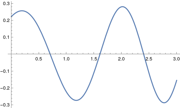
It is known that differential equation (7.1) has two linearly independent solutions y₁(x) = cos(x) and y₂(x) = sin(x) through which the general solution is expressed. However, we are going to show how their properties can be squeezed out of differential equation (7.1) and corresponding initial conditions.
sin = Plot[Sin[x], {x, 0, 6}, PlotStyle -> {Dashed, Thick, Black}, PlotRange -> {{-0.2, 6.5}, {-1.1, 1.1}}, Axes -> False];
cos = Plot[Cos[x], {x, 0, 6}, PlotStyle -> {Thick, Blue}, PlotRange -> {{-0.2, 6.5}, {-1.1, 1.1}}, Axes -> False];
ax = Graphics[{Thick, Arrow[{{-0.2, 0}, {2*Pi, 0}}]}];
ay = Graphics[{Thick, Arrow[{{0, -3.2}, {0, 3.2}}]}];
tsin = Graphics[{Black, Text[Style["sin x", 18], {6.3, -0.45}]}];
tcos = Graphics[{Blue, Text[Style["cos x", 18], {6.1, 1.1}]}];
tx = Graphics[{Blue, Text[Style["x", 18], {6.7, 0.2}]}];
ty = Graphics[{Blue, Text[Style["y", 18], {0.2, 1.15}]}];
line = Graphics[{Dashed, Thick, Line[{{Pi/2, 0}, {Pi/2, 1}}]}];
tm = Graphics[{Blue, Text[Style["m", 18], {Pi/2, -0.2}]}];
disk = Graphics[{Orange, Disk[{Pi/2, 0}, 0.05]}];
Show[sin, cos, tsin, tcos, ax, ay, tx, ty, line,tm,disk]
Two linearly independent solutions

Accordingly, let y = c(x) be the solution of Eq.(7.1) subject to the initial conditions y(0) = 1, y'(0) = 0, and y = s(x) be defined as the solution of Eq.(7.1) determined by the 
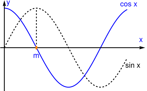
initial conditions s(0) = 0 and s′(0) = 1. If we try to sketch the graphs of these functions, we know from the initial conditions that s(x) starts from the origin, but c(x) starts from point (0,1). We know that s(x) is increasing because its derivative at the origin is 1 (positive). From the equation itself we have s″(x) = −s(x), so when the curve is above the x-axis, s″(x) is a negative number that increases in magnitude as the curve rises. Since s″(x) is the rate of change of the slope s′(x), this slope decreases at an increasing rate as the curve lifts, and it must reach 0 at some point x = m. As x continues to increase, the curve falls toward the x-axis, s′(x) decreases at a decreasing rate, and the curve crosses the x-axis at a point we can define to be π. Since s″(x) depends only on s(x), we see that the graph between x = 0 and x = π is symmetric about the line x = m, so m = π/2 and s′(π) = −1. A similar argument shows that the next portion of the curve is an inverted replica of the first arch, and so on indefinitely.

On the other hand, slope of c(x) beginning at 0. since by equation (7.1) we know that c″(x) = –c(x), the same reasoning as before shows that the curve bends down and crosses the x-axis. It is natural to conjecture that the height of the first arch of s(x) is 1, that the first zero of c(x) is π/2, etc.; but to establish these guesses as facts, we begin by showing that

\[ s' (x) = c(x) \qquad\mbox{and} \qquad c' (x) = -s(x) . \tag{7.2} \]
To prove the first statement, we start by observing that (7.1) yields y‴+ y′ = 0 or (y′)″ + y′ = 0, so the derivative of any solution of (7.1) is again a solution. Thus, s′(x) and c(x) are both solutions of (7.1), and it suffices to show that they have the same values and the same derivatives at x = 0. This follows at once from s′(0) = 1, c(0) = 1 and s″(0) = –s(0) = 0, c′(0) = 0. The second formula in (7.2) is an immediate consequence of the first, for c′(x) = s″(x) = –s(x). We now use (7.2) to prove
\[ c(x)^2 + s(x)^2 = 1. \tag{7.3} \]
Since the derivative of the left side of (7.3) is
\[ 2s(x)\,c(x) - 2c(x) \,s(x) , \]
which is 0, we see that s(x)² + c(x)² equals a constant, and this constant must be 1 because s(0)² + c(0)² = 1. It follows at once from (7.3) that the height of the first arch of s(x) is 1 and that the first zero of c(x) is π/2. This result also enables us to show that s(x) and c(x) are linearly independent, for their Wronskian is
\[ W\left[ c(x), s(x) \right] = c(x)\,s' (x) - s(x)\,c' (x) = c(x)^2 + s(x)^2 = 1 \ne 0. \]
In much the same way, we can continue and establish the following additional facts:
\begin{align*} c(x+y) &= c(x)\,c(y) - s(x)\,s(y) , \\ s(x+y) &= s(x)\,c(y) + c(x)\,s(y) , \\ s(2x) &= 2\,s(x)\, c(x) , \\ c(2x) &= c(x)^2 - s(x)^2 , \\ s(x+ 2\pi ) &= s(x) \end{align*}
Among other things, it is easy to see from the above results that the positive zeros of s(x) and c(x) are, respectively, π, 2π, 3π, . . . and π/2, π/2 + π, π/2 + 2π, . . . .

<[> There are two main points to be made about the above discussion. First, we have extracted almost every significant property of the functions sin x and cos x from equation (7.1) by the methods of differential equations alone, without using any prior knowledge of trigonometry. Second, the tools we did use consisted chiefly of convexity arguments (involving the sign and magnitude of the second derivative) and the basic properties of linear equations set forth.

It goes without saying that most of the above properties of sin x and cos x are peculiar to these functions alone. Nevertheless, the central feature of their behavior—the fact that they oscillate in such a manner that their zeroes are distinct and occur alternately—can be generalized far beyond these particular functions.

End of Example 7
   ■

Sturm’s Comparison Theorem: For i = 1,2, let ui(x) be a nontrivial solution of the differential equation \( \displaystyle \left( p_i(x)\, u'_i \right)' + q_i u_i = 0 \) on α ≤ x ≤ β. Suppose further that the coefficients are continuous and for x ∈ [α, β]

\( q_2 (x) \ge q_1 (x) , \quad \) with \( \quad q_2 (x_0 ) > q_1 (x_0 ) \quad \) for some x0,     \( p_2 (x) \le p_1 (x) . \quad \)

Then if α, β are two consecutive zeros of u1(x), the open interval (α, β) will contain at least one zero of u2(x).
It was Mauro Picone who in 1909 disposed of the case p₁ ≠ p₂.

For simplicity, we denote by u and v eigenfunctions corresponding i₁ and i₂, respectively.

Suppose to the contrary that v does not vanish in (&alha;, β). It may be supposed without loss of generality that v(x) > 0 and also u(x) > 0 in (&alha;, β). Multiplication of the equation

\[ \ell\left[ x, \texttt{D} \right] u = \frac{text d}{{\text d}x} \left( p(x)\,\frac{{\text d}u}{{\text d}x} \right) + q_1 (x)\,u =0 \]
by v(x) and the equation
\[ L\left[ x, \texttt{D} \right] v = \frac{text d}{{\text d}x} \left( p(x)\,\frac{{\text d}v}{{\text d}x} \right) + q_2 (x)\,v =0 \]
by u(x) and then subtraction of the resulting equations, and integration over (&alha;, β) yields
\[ \int_{\alpha}^{\beta} \left[ \left( p\,u' \right)' v - \left( p\,v' \right)' u \right] {\text d}x = \int_{\alpha}^{\beta} \left[ (q_1 - q_2 )\,uv \right] {\text d}x \]
Since the integrand on the left side is the derivative of \( p(x)\, W[u,v) = p \left( u' v - v' u \right) , \) and q₁ > q₂ by hypothesis, it follows that
\[ \left[ p(x)\, u' (x) v(x) - p(x)\,v' (x)\,u(x) \right]_{x=\alpha}^{x=\beta} > 0 . \tag{P.1} \]
However, u(α) = u(β) = 0 by hypothesis, and since u(x) > 0 in (α, β), u'(α) > 0 and u'(β) < O. Thus the left member of Eq.(P.1) is negative, which is a contradiction.
Sturm’s proofs of course do not meet the standards of modern rigor. They meet the standards of his time, and are in fact correct in method and can without too much trouble be made rigorous. The first efforts to do this are due to Maxime Bôcher in a series of papers in the Bulletin of the AMS and are also contained in his book. Bôcher remarks that “the work of Sturm may, however, be made perfectly rigorous without serious trouble and with no real modification of method”. The conditions placed on the coefficients were to make them piecewise continuous. Bôcher used Riccati equation techniques in some of his proofs; it should be noted that Sturm mentions the Riccati equation, but does not employ it in his proofs. Riccati equation techniques in variational theory go back at least to Legendre who in 1786 gave a flawed proof of his necessary condition for a minimizer of an integral functional. A correct proof of Legendre’s condition using Riccati equations can be found in Bolza’s 1904 lecture notes. Bolza attributes this proof to Weierstrass.

  • Bôcher. M., The theorems of oscillation of Sturm and Klein, Bull. Amer. Math. Soc. 4 (1897–1898), 295–313, 365–376.
  • Bôcher, M., Leçons sur les méethodes de Sturm dans la théorie des équations différentielles linéaires, et leurs déeveloppements modernes, Gauthier-Villars, Paris, 1917.
  • Bolza, O., Lectures on the Calculus of Variations, Dover, New York, 1961.

Example 8: 
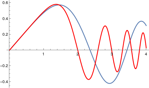
Let us consider two differential equations and corresponding initil conditions

\[ u'' + x^2 u = 0 \qquad u(0) = 0, \quad u' (0) = 0.5; \tag{8.1} \]
and
\[ v'' + x^4 v = 0 \qquad v(0) = 0, \quad v' (0) = 0.5. \tag{8.2} \]
Since these initial value problems are impossible to solve analytically, we apply Mathematica and its dedicated command NDSolve for numerical approximation.
sol2 = NDSolve[{y''[x] + x^2 *y[x] == 0, y[0] == 0, y'[0] == 0.5}, y, {x, 0, 10}];
y2 = Plot[Evaluate[y[x] /. sol2], {x, 0, 4}, PlotStyle -> Thick]
sol4 = NDSolve[{u''[x] + x^4*u[x] == 0, u[0] == 0, u'[0] == 0.5}, u, {x, 0, 4}];
u4 = Plot[Evaluate[u[x] /. sol4], {x, 0, 4}, PlotStyle -> {Red, Thick}]
Show[y2, u4]
Two oscilating solutions

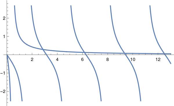
As it is seen from the graph, between any two zeroes of u(x), there is always a zero of v(x), but not vice versa.
End of Example 8
   ■


Sturm--Liouville problem with periodic conditions


Another important class of Sturm--Liouville problems provide second order differential equations with periodic boundary conditions. As an example, we consider the eigenvalue problem
\begin{equation} \label{EqSturm.7} y'' + \lambda \,y =0 , \qquad y(0) = y(T) , \qquad y' (0) = y'(T) . \end{equation}
We are going to show that eigenvalues of this Sturm--Liouville problem with periodic conditions possess almost all properties as regular Sturm--Liouville problems, except that they are not simple having multiplicity two. You will observe the difference in behavior of the eigenvalues between the regular Sturm--Liouville problem and periodic problems is due to the fact that the eigenvalues of a regular problem are simple, whereas for the periodic case they can have multiplicity two.

Although Sturm--Liouville problems with periodic conditions provide different kind of conditions compared to problems with homogeneous boundary conditions, it can be analyzed in a similar way as we did for regular eigenvalue/eigenfunction problems. First observation that you need to make is to prove that the operator generated by periodic conditions \eqref{EqSturm.7} is self-adjoint. Thus, we have to demonstrate the validity of the following identity:

\[ \left\langle L\left[ \texttt{D} \right] u , v \right\rangle = \left\langle u , L\left[ \texttt{D} \right] v \right\rangle \qquad \mbox{or} \qquad \left\langle L\left[ \texttt{D} \right] u , v \right\rangle - \left\langle u , L\left[ \texttt{D} \right] v \right\rangle = 0 \]
for any two functions u and v from the domain of the corresponding operator. This means that these functions have two first continuous derivatives and satisfy the periodic conditions.

Using integration by parts and Lagrange's identity, we get

\[ \left\langle L\left[ \texttt{D} \right] u , v \right\rangle - \left\langle u , L\left[ \texttt{D} \right] v \right\rangle = \int_0^T \frac{\text d}{{\text d}x} \left[ p(x) \left( v\, \frac{{\text d}u}{{\text d}x} - u \,\frac{{\text d}v}{{\text d}x}\right) \right] {\text d}x = \left[ p(x) \left( v\, \frac{{\text d}u}{{\text d}x} - u \,\frac{{\text d}v}{{\text d}x}\right) \right]_{x=0}^{x=T} . \]
Because of periodic conditions
\[ \left[ p(x) \left( v\, \frac{{\text d}u}{{\text d}x} - u \,\frac{{\text d}v}{{\text d}x}\right) \right] (x=0) = \left[ p(x) \left( v\, \frac{{\text d}u}{{\text d}x} - u \,\frac{{\text d}v}{{\text d}x}\right) \right] (x=T) , \]
and the operator becomes self-adjoint. Therefore, we expect that the Sturm--Liouville problem with periodic conditions has only real eigenvalues and its corresponding eigenfunctions are orthogonal.

Solutions of the differential equation \( y'' + \lambda \,y =0 \) depend on the sign of parameter λ. If λ = −μ2 is negative, the equation has two exponential linearly independent solutions \( y_1 = e^{\mu x} \quad\mbox{and}\quad y_2 = e^{-\mu x} \) that also sometimes can be written through hyperbolic sine and cosine functions. These functions cannot be periodic, so negative λ is not an eigenvalue.

If λ = 0, the general solution of the differential equation \( y'' =0 \) is a linear function \( y = a + b\,x , \) which could be periodic only when b = 0. So zero is an eigenvalue corresponding to an eigenfunction which is a constant function in this case.

When λ = ω2 is positive, then the general solution becomes

\[ y = a\,\cos (\omega x) + b\,\sin (\omega x) , \]
with some constants 𝑎 and b. This function is periodic with period T if and only if ω is proportional to 2π/T; so we get eigenvalues
\[ \omega_n = \frac{2n\pi}{T} \qquad \Longrightarrow \qquad \lambda_n = \left( \frac{2n\pi}{T} \right)^2 , \quad n= 1,2,3,\ldots . \]
The corresponding linearly independent eigenfunctions are
\[ \cos \frac{2n\pi x}{T} \qquad\mbox{and} \qquad \sin \frac{2n\pi x}{T} , \quad n=1,2,3,\ldots . \]
Therefore, the eigenspace is two-dimensional and the eigenfunction can be written in vector form:
\begin{equation*} \phi_n (x) = \left[ \begin{array}{c} \cos \left( \frac{2n\pi x}{T} \right) \\ \sin \left( \frac{2n\pi x}{T} \right) \end{array} \right] , \qquad n=0,1,2,\ldots . \end{equation*}
We can include λ = 0 into the general formula and claim that Sturm--Liouville problem \eqref{EqSturm.7} has a sequence of nonnegative eigenvalues
\begin{equation*} \lambda_n = \left( \frac{2n\pi}{T} \right)^2 , \qquad n=0,1,2,3,\ldots ; \end{equation*}
with corresponding eigenfunctions
\[ \phi_n (x) = a_n \cos \left( \frac{2n\pi x}{T} \right) + b_n \sin \left( \frac{2n\pi x}{T} \right) , \]
where 𝑎n, bn are some real constants. These arbitrary constants indicate that the eigenfunction is two-dimensional. Of course, you can organize it in one-dimensional array upon introducing positive and negative indices:
\[ \phi_n (x) = \cos \left( \frac{2n\pi x}{T} \right) , \quad n=0,1,2,\ldots ; \qquad \phi_{-n} (x) = \sin \left( \frac{2n\pi x}{T} \right) , \quad n=1, 2, 3 , \ldots . \]
Then setting 𝑎-n = bn, we utilize a one-dimensional list.
\[ \left[ \cdots , \sin \left( \frac{2\pi nx}{T} \right) , \cdots , \sin \left( \frac{4\pi x}{T} \right) , \sin \left( \frac{2\pi x}{T} \right) , 1, \ \cos \left( \frac{2\pi x}{T} \right) , \cos \left( \frac{4\pi x}{T} \right) , \cdots , \cos \left( \frac{2\pi nx}{T} \right) , \cdots , \right] . \]


Observe that the differential operator \( -\texttt{D}^2 \) in Sturm--Liouville problem \eqref{EqSturm.7} is a square of another differential operator of order one: \( \quad -\texttt{D}^2 = \left( -{\bf j}\texttt{D} \right)^2 . \) Correspondingly, we consider a Sturm--Liouville problem for first order differential operator:
\begin{equation*} \left( {\bf j} \right) \psi' + \mu \,\psi =0 , \qquad y(0) = y(T) . \end{equation*}
Its general solution is spanned on
\[ \psi (x) = e^{-{\bf j}\,\mu x} . \]
To satisfy the periodic conditions, we have to set \( \mu = 2n\pi /T , \) with n = 0, ±1, ±2, ….

Example 9: Now we consider another Sturm--Liouville problem with anti-periodic boundary conditions

\[ y'' + \lambda \,y =0 , \qquad y(-\ell ) = -y(\ell ) , \qquad y' (-\ell ) = - y'(\ell ) . \tag{A1.1} \]
Following the previous example, it is clear that the given anti-periodic problem has a nontrivial solution only when &lambda is positive; so we let λ = μ². Then the general solution of the differential equation (A1.1) is
\[ y(x) = a\,\cos \mu x + b\,\sin \mu x , \]
for some constants 𝑎 and b. To satisfy the anti-periodic conditions, we should have
\[ \cos \mu\ell = - \cos \mu\ell \qquad\mbox{and} \qquad \sin \left(- \mu\ell \right) = - \sin \mu\ell . \]
The latter condition is satisfies automatically (because sine function is odd). However, the former requires
\[ \cos \mu\ell = 0 \qquad \Longrightarrow \qquad \mu\ell = \left( n + \frac{1}{2} \right) \pi , \quad n=0,1,2,\ldots . \]
Therefore, the given Sturm--Liouville problem with anti-periodic conditions has infinite many eigenfunctions:
\[ \phi_n (x) = a_n \cos\left( n + \frac{1}{2} \right) \frac{\pi x}{\ell} + b_n \sin \left( n + \frac{1}{2} \right) \frac{\pi x}{\ell} , \qquad n=0,1,2,\ldots . \]
This eigenfunction relects that the eigenvalue has multiplicity two.    ■


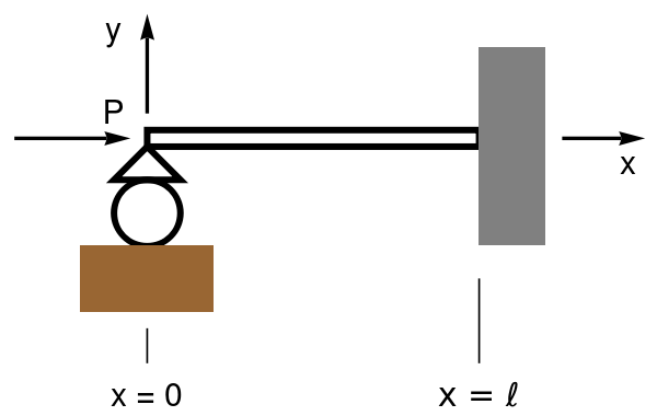
Buckling of an Elastic Column


We consider a buckling problem as an example of boundary value problems that lead to the fourth order differential equations. Therefore, we consider an elastic column of length ℓ, one end ot it is clumped, but another one is simply supported. Let y(x) be the deflection of the column at point x from its equilibrium position.

The bending moment M = P yH x = −E I y'', where H is the horizontal force of reaction, and P is a load. Here E is Young's modulus and I is the moment of inertia of the cross section about an axis through the centroid perpendicular to he plane. Upon differentiation, we get

\[ \left( EI\,y'' \right)'' = P\,y'', \qquad y(0) = y'' (0) =0, \quad y(\ell ) = y'(\ell ) = 0. \]
The boundary conditions at x = 0 and x = ℓ depend on how the ends of the column are supported. Typical boundary conditions are
\begin{align*} y = y' =0, \qquad &\mbox{clamped end}, \\ y = y'' =0, \qquad &\mbox{simply supported (hinged) end}. \end{align*}
If
flexural rigidity EI is a constant, we set k² =P/(EI), with units m−2, and get the Sturm–Liouville problem
\[ y^{(iv)} + k^2 y'' =0, \qquad y(0) = y'' (0) =0, \quad y(\ell ) = y'(\ell ) = 0. \]

The general solution of the forth order differential equation \( y^{(iv)} + k^2 y'' =0 \) is

\[ y (x) = a + bx + c\,\cos kx + d\, \sin kx, \]
with some constants 𝑎, b, c, and d. The boundary conditions dictate that 𝑎 = c = 0, and the eigenvalues kn (n = 1, 2, 3, …) are roots of the transcendent equation
\[ \sin (k\ell ) = k\ell\,\cos (k\ell ). \]
The eigenfunctions corresponding to the eigenvalues are
\[ y_n (x) = \sin (k_n x) - x k_n \cos (k_n \ell ) , \qquad n=1,2,3,\ldots . \]
When k = 0, the general solution becomes \( y = a + bx + c x^2 + d x^3 . \) The boundary conditions are satisfied only when 𝑎 = b = c = d = 0. Hence λ = 0 is not an eigenvalue.
rod = Graphics[{Thickness[0.01], Line[{{0, 0}, {1.0, 0}, {1.0, 0.05}, {0, 0.05}, {0, 0}}]}];
tri = Graphics[{Thickness[0.01], Line[{{0, 0}, {-0.1, -0.1}, {0.1, -0.1}, {0, 0}}]}];
circle = Graphics[{Thickness[0.01], Circle[{0, -0.2}, 0.1]}];
ground = Graphics[{Brown, Rectangle[{-0.2, -0.3}, {0.2, -0.5}]}];
wall = Graphics[{Gray, Rectangle[{1, 0.3}, {1.2, -0.3}]}];
ay = Graphics[{Thick, Arrow[{{0, 0.1}, {0, 0.4}}]}];
ax = Graphics[{Thick, Arrow[{{1.25, 0.025}, {1.5, 0.025}}]}];
l1 = Graphics[{Line[{{0.0, -0.55}, {0.0, -0.65}}]}];
l2 = Graphics[{Line[{{1.0, -0.4}, {1.0, -0.65}}]}];
tl = Graphics[{Black, Text[Style["x = \[ScriptL]", 18, FontFamily -> "Mathematica1"], {1.0, -0.75}]}];
t0 = Graphics[{Black, Text[Style["x = 0", 18], {0.0, -0.75}]}];
tx = Graphics[{Black, Text[Style["x", 18], {1.45, -0.05}]}];
ty = Graphics[{Black, Text[Style["y", 18], {-0.1, 0.35}]}];
tp = Graphics[{Black, Text[Style["P", 18], {-0.1, 0.1}]}];
Show[rod, tri, circle, ground, wall, ay, ax, ap, l1, l2, t0, tl, tx, \ ty, tp]
\
Backling of an elastic column.


Euler Buckling


Suppose that a straight elastic bar (beam, rod, or column) of length ℓ is positioned horizontally and is anchored at its base. Experimentally one can take a thick metal wire. A small compressive force of magnitude P acts horizontally on pin ended column. downward on the free end of the bar as in Figure 1.1. The equation governing the shape of the bar is
\[ E\,I\,\frac{{\text d}^2 w}{{\text d} x^2} + P\,w = 0, \]
where w is the lateral deflection. Let \( \lambda^2 = P/(EI) , \) using the boundary consditions, we obtaine the Sturm--Liouville problem:
\[ w'' + \lambda^2 w = 0, \qquad w(0) = 0, \quad w(\ell ) = 0. \]
Euler's critical load is the compressive load at which a slender column will suddenly bend or buckle. It is given by the formula tat was derived in 1757 by Leonhard Euler:
\[ P_{cr} = \frac{\pi^2 E\.I}{(K\ell )^2} , \]
where
  • Pcr is Euler's critical load (longitudinal compression load on column),
  • E is Young's modulus of the column material (usually expressed in gigapascals),
  • I is minimum area moment of inertia of the cross section of the column (second moment of area),
  • ℓ, unsupported length of column or rod,
  • K is column effective length factor.
If buckling occurs, it must be possible to find a solution (or solutions) to the governing equations different from the obvious solution w(x) = 0 for 0 ≤ x ≤ ℓ, the so-called trivial solution. Other solutions, if any exist, are called nontrivial. They are
\[ w(x) = A\,\sin \left( \frac{\pi x}{\ell} \right) , \]
with some nonzero constant A. The smallest eigenvalue determines the minimum compressive force needed to buckle a beam of given flexural rigidity EI.

The Euler model predicts that buckling can occur and does occur only at the eigenvalues λn and that the corresponding buckled equilibrium states are multiples of sin(nπx/&ell:). Actually, once the bar has buckled, a new model is needed because the physical situation has become nonlinear. Nevertheless, even in the nonlinear regime the linear problem above, which is the linearization of an appropriate nonlinear model, still predicts the values of P at which buckling can occur. Problems of this sort are called bifurcation (branching) problems because nonlinear states branch from a stable linear state at certain critical values, the eigenvalues of the linearized problem. The eigenfunction wn corresponding to the branch point determined by the eigenvalue λn approximates the shape of the nonlinear buckled responses of small amplitude that occur near the branch point.

  1. Guenther, R.B. and Lee, J.W., Sturm-Liouville Problems Theory and Numerical Implementation, 2018, CRC Press.
  2. Li H. and Torney D., A complete system of orthogonal step functions, Proceedings of The American mathematical Society, Vol. 132, No 12, pp. 3491--3504.
  3. Lützen, J., Sturm and Liouville's Work on Ordinary Linear Differential Equations. The Emergence of Sturm-Liouville Theory, online.
  4. Simmons, G.F., Differential Equations with Applications and Historical Notes, Third edition, CRC Press, Boca Raton, London, New York.
  5. Swanson, C.A., Comparison and oscillation theory of linear differential equations, Academic Press, New York and London, 1968.
  6. Titchmarsh, E.C., Eigenfunction expansions associated with second-order differential equations I, Clarendon Press, Oxford, 1962.
  7. Whittaker, E.T. and Watson, G.N., Modern analysis, Cambridge University Press, 1950
  8. Zettl, A., Computing continuous spectrum, in Trends and Developments in Ordinary Differential Equations, 393–406, Y. Alavi and P. Hsieh editors, World Scientific, 1994.
  9. Zettl, A., Sturm-Liouville problems, in Spectral Theory and Computational Methods of Sturm-Liouville problems, 1–104, Lecture Notes in Pure and Applied Mathematics 191, Marcel Dekker, Inc., New York, 1997.


Some utube references:
  1. Convert the differential equation \( y'' + x\,y' + 3\, y =0 \) to a self-adjoint form.

    Answer: \( \mu = e^{x^2 /2} . \)

  2. Show that the substitution \( y = x^{-1/2} z \) reduces Bessel's equation of order ν
    \[ x^2 y'' + x\,y' + \left( x^2 - \nu^2 \right) y = 0 \]
    to the form
    \[ z'' + \left( x^2 + \frac{1}{4} - \nu^2 \right) x^{-2} z = 0. \]
  3. Reduce the following differential equations to self-adjoint form:
    1. \( \displaystyle \left( 1 - x^2 \right) y'' - x\,y' + \lambda\, y = 0 ; \)     (Chebyshev equation);
    2. \( \displaystyle \left( 1 - x^2 \right) y'' - 2x\,y' + \lambda\, y = 0 ; \)     (Legendre equation);
    3. \( \displaystyle x^2 y'' + x\,y' + \lambda\, y = 0 ; \)     (Euler equation);
    4. \( \displaystyle x^2 y'' + y' \,\tan x = 0 ; \)
  4. For each of the following differential equations, y = x³ is one solution; find a second, linearly independent solution by quadratures.
    1. \( \displaystyle x^2 y'' - 4x\,y' + 6\, y = 0 ; \)
    2. \( \displaystyle x\, y'' - \left( x-2 \right) y' - 3\, y = 0 . \)
  5. Consider the Sturm--Liouville problem
    \[ y'' + \lambda\,y = 0, \qquad y(0) - h\,y' (0) = 0, \qquad y' (1) = 0, \]
    where h is a given parameter.
    1. Show that for all real values of parameter h there is an infinite sequence of positive eigenvalues
    2. Show that the principal eigenvalue (a smallest one) approaches zero as h approaches infinity. Show that the principal eigenvalue approaches π/2 as h approaches zero from above.
    3. Show that λ = 0 is not an eigenvalue for any h.
    4. Show that the given SL problem has negative eigenvalues iff h < 0.
  6. Answer:
    1. Suppose that λ < 0, then denoting −λ = μ², we get the general solution of \( y'' - \mu^2 y = 0 \) is
      \[ y = c_1 \cosh (\mu x) + c_2 \sinh (\mu x) . \]
      From the boundary condition at x = 0, we get c₁ = μch. Using this value, we obtain from another boundary condition at x = 1 that
      \[ \mu h\,\sinh (\mu ) + \cosh (\mu ) = 0 \qquad \longrightarrow \qquad - \mu h = \coth (\mu ) = \frac{\cosh \mu}{\sinh \mu} \]
      Upon plotting these two functions, we see that they do not intersect; therefore, λ < 0 is not an eigenvalue.
      Plot[{-0.5*m, Coth[m]}, {m, -3, 3}, PlotStyle -> Thick]

      If λ = 0, the general solution of \( y'' = 0 \) is q linear function c₁ + cx. From the boundary condition at x = 1, it follows that c₂ = 0. Another boundary condition at the origin leads to c₁ = 0. Therefore, λ = 0 is not an eigenvalue.

      Assuming λ = &mu² > 0, we have the general solution

      \[ y = c_1 \cos (\mu x) + c_2 \sin (\mu x) . \]
      The boundary conditions yield
      \begin{align*} c_1 - \mu c_2 h &= 0 \qquad \longrightarrow \qquad c_1 = \mu c_2 h, \\ -c_1 \sin \mu + c_2 \cos \mu &= 0 \qquad \longrightarrow \qquad \mu h\, \sin \mu = \cos \mu . \end{align*}
      This leads to the transcendent equation
      \[ \mu h = \cot \mu = \frac{\cos \mu}{\sin \mu} . \]
      Upon plotting two functions, we see that that there are infinite many eigenvalues.
      Plot[{1.5*m, Cot[m]}, {m, 0, 20}, PlotStyle -> Thick]
      with \( \mu_n \approx n\pi \) for large n.
    2. When h grows, the straight line hμ has larger slope that crosses cotangent curve near the origin.

      When h approaches zero , the straight line hμ becomes closer to the abscissa that crosses the cotangent curve at μ = π/2.

    3. It was shown previously that λ = 0 is not an eigenvalue for any h. Show that λ = 0 is an eigenvalue only when h = 1.
    4. From the graph
      Plot[{-1.5*m, Cot[m]}, {m, 0, 20}, PlotStyle -> Thick]
      it is obvious that the straight line with negative slope crosses the cotangent line in the fourth quadrant.
  7. Consider the eigenvalue problem for transverse vibration of an uniform elastic bar:
    \[ y^{(4)} + \lambda\,y = 0, \qquad y(0) - h\,y' (0) = 0, \qquad 0 < x < \ell , \]
    where y is the transverse displacement and λ = mω²/(EI); m is the mass per unit length of the rod, E is Young's modulus, I is the moment of inertia of the cross section about an axis through the centroid perpendicular to the plane of vibration, and ω is the frequency of vibration. Hence, for a bar whose material and geometrical properties are given, the eigenvalues determine the natural frequencies of vibration. Boundary conditions at each end are usually one of the following types"
    \begin{align*} & y = y' = 0 \qquad \mbox{clamped end}, \\ & y = y'' = 0, \qquad \mbox{simply supported or hinged end}, \\ & y'' = y''' = 0, \qquad \mbox{free end}. \end{align*}
    For each of the following three cases, find the form of the eigenfunctions and the equation satisfied by the eigenvalues of this fourth order boundary value problem. Determine λ₁ and λ₂, the two eigenvalues of smallest magnitude. Assume that the eigenvalues are real and positive.
    1. y(0) = y'(0) = 0,      y(ℓ) = y''(ℓ) = 0;
    2. y(0) = y''(0) = 0,      y(ℓ) = y'(ℓ) = 0;
    3. y(0) = y'(0) = 0,      y''(ℓ) = y'''(ℓ) = 0      (cantilevered bar).