Preface
This section studies some first order nonlinear ordinary differential equations describing the time evolution (or “motion”) of those hamiltonian systems provided with a first integral linking implicitly both variables to a motion constant. An application has been performed on the Lotka--Volterra predator-prey system, turning to a strongly nonlinear differential equation in the phase variables.
Return to computing page for the first course APMA0330
Return to computing page for the second course APMA0340
Return to Mathematica tutorial for the first course APMA0330
Return to Mathematica tutorial for the second course APMA0340
Return to the main page for the first course APMA0330
Return to the main page for the second course APMA0340
Return to Part III of the course APMA0340
Introduction to Linear Algebra with Mathematica
Glossary
Limit Cycles
Consider a system of first order autonomous ordinary differential equations in normal form
If an initial position of the vector \( {\bf x} (t) \) is known, we get an initial value problem:
2.3.5. Limited Circles
- g(x) > 0 for all x > 0;
- \( \lim_{x\to \infty} F(x) \equiv \lim_{x\to \infty} \int_0^x f(\xi )\,{\text d}\xi = \infty ; \)
- F(x) has exactly one positive root at some value p, where F(x) < 0 for 0 < x < p and F(x) > 0 and monotonic for x > p.
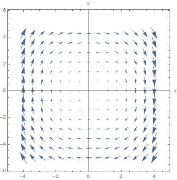
Axes -> True, AspectRatio -> 1, VectorPoints -> 15, AxesLabel -> {x, v}]
Module[{xans, vans},
{xans, vans} = {x[t], v[t]} /. Flatten[NDSolve[duff[x0, v0], {x[t], v[t]}, {t, 0, 8}]];
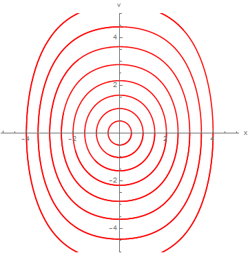
ParametricPlot[{xans, vans}, {t, 0, 8}, PlotRange -> {{-5.1, 5.1}, {-5, 5}},
AxesLabel -> {"x", "v"}, AspectRatio -> 1, DisplayFunction -> Identity,
PlotStyle -> RGBColor[1, 0, 0]]];
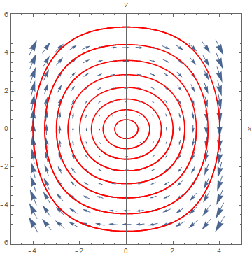
Do[pair = initlist[[i]];
x0temp = First[pair]; v0temp = Last[pair]; newgraph = graph[x0temp, v0temp];
graphlist = Append[graphlist, newgraph], {i, 1, 8}]]
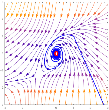 |
StreamPlot[{-y - x^2, 2*x - y^3}, {x, -2.5, 2.5}, {y, -2.5, 2.5},
StreamScale -> Large]
|
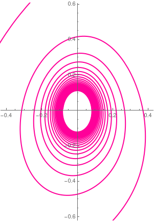 |
A = StreamPlot[{-y - x^2, 2*x - y^3}, {x, -2.5, 2.5}, {y, -2.5, 2.5},
StreamScale -> Large, PlotRange -> {{3, -3}, {3, -3}}];
sol = NDSolve[{x'[t] == -y[t] - (x[t])^2, y'[t] == 2*x[t] - (y[t])^3, x[0] == 1, y[0] == 1}, {x, y}, {t, 0, 150}]; B = ParametricPlot[Evaluate[{x[t], y[t]} /. sol], {t, -.1, 100}, PlotStyle -> {Blue, Thick}, PlotRange -> {{3, -3}, {3, -3}}] ; B2 = ParametricPlot[Evaluate[{x[t], y[t]} /. sol], {t, 95, 100}, PlotStyle -> {Red, Thickness[.012]}, PlotRange -> {{3, -3}, {3, -3}}]; Show[A, B, B2, PlotRange -> {{3, -3}, {3, -3}}] Show[A, B, B2, PlotRange -> {{.5, -.5}, {.5, -.5}}] |
|
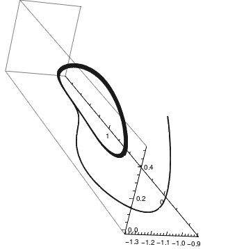
We plot solutions to RF system when α = 1.14 and γ = 0.1 with the initial conditions
\[
x(0) = -1, \quad y(0) = 0, \quad z(0) = 0.5.
\]
The corresponding limit circle (in red color) is clearly visible.
a = 1.14; gamma = 0.1;
sol = NDSolve[{x'[t] == y[t]*(z[t] - 1 + (x[t])^2) + gamma*x[t], y'[t] == x[t]*(3*z[t] + 1 - (x[t])^2) + gamma*y[t], z'[t] == -2*z[t]*(a + x[t]*y[t]), x[0] == -1, y[0] == 0, z[0] == 0.5}, {x, y, z}, {t, 0, 200}]; pp = ParametricPlot3D[ Evaluate[{x[t], y[t], z[t]} /. sol], {t, 0, 100}, PlotRange -> All, PlotTheme -> "Monochrome"]; lim = ParametricPlot3D[ Evaluate[{x[t], y[t], z[t]} /. sol], {t, 35, 100}, PlotRange -> All, PlotTheme -> "Monochrome", PlotStyle -> {Red, Thickness[.005]}]; Show[lim, pp] |
|
| Rabinovich–Fabrikant system | Mathematica code |
■
2.3.6. Applications
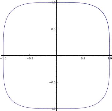
G[x_, y_] := x^3;
sol = NDSolve[{x'[t] == F[x[t], y[t]], y'[t] == G[x[t], y[t]],
x[0] == 1, y[0] == 0}, {x, y}, {t, 0, 3*Pi},
WorkingPrecision -> 20]
ParametricPlot[Evaluate[{x[t], y[t]}] /. sol, {t, 0, 3*Pi}]
{{x -> InterpolatingFunction[{{0, 9.4247779607693797154}}, <>],
y -> InterpolatingFunction[{{0, 9.4247779607693797154}}, <>]}}
Y[t_] := Evaluate[y[t] /. sol]
fns[t_] := {X[t], Y[t]};
len := Length[fns[t]];
Plot[Evaluate[fns[t]], {t, 0, 3*Pi}]
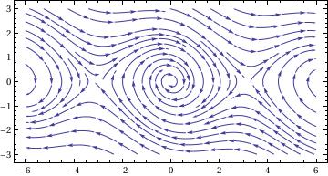
V. Pendulum Equation
fx = Function[{x, y}, y]; fy = Function[{x, y}, -Sin[x] - 0.25*y]
portrait =
StreamPlot[{fx[x, y], fy[x, y]}, {x, -6, 6}, {y, -3, 3},
AspectRatio -> Automatic]
solution =
Function[point,
Function @@ {t, ({x[t], y[t]} /.
NDSolve[{x'[t] == fx[x[t], y[t]], y'[t] == fy[x[t], y[t]],
Thred[{x[time], y[time]} == point]}, {x, y}, {t, time,
time + 40}])[[1]]}]
Out[12]=
Function[point,
Function @@ {t, ({x[t], y[t]} /.
NDSolve[{Derivative[1][x][t] == fx[x[t], y[t]],
Derivative[1][y][t] == fy[x[t], y[t]],
Thred[{x[time], y[time]} == point]}, {x, y}, {t, time,
time + 40}])[[1]]}]
V. van der Pol Equation
- D’Acunto M., Determination of limit cycles for a modified van der Pol oscillator. Mechanics Research Communications, 2006, 33:93–100. [doi:10.1016/j.mechrescom.2005.06.012]
- Gottlieb, H.P.W., 2006. Harmonic balance approach to limit cycles for nonlinear jerk equations. Journal of Sound and Vibration, 297:243–250. [doi:10.1016/j.jsv.2006.03.047]
- He, J.H., 2003. Determination of limit cycles for strongly nonlinear oscillators. Physical Review Letters, 90(17), Article No. 174301.
- He, J.H., 2006a. Determination of limit cycles for strongly nonlinear oscillators. Physic Review Letter, 90:174–181.
Return to Mathematica page
Return to the main page (APMA0340)
Return to the Part 1 Matrix Algebra
Return to the Part 2 Linear Systems of Ordinary Differential Equations
Return to the Part 3 Non-linear Systems of Ordinary Differential Equations
Return to the Part 4 Numerical Methods
Return to the Part 5 Fourier Series
Return to the Part 6 Partial Differential Equations
Return to the Part 7 Special Functions