Preface
This tutorial was made solely for the purpose of education and it was designed for students taking Applied Math 0340. It is primarily for students who have some experience using Mathematica. If you have never used Mathematica before and would like to learn more of the basics for this computer algebra system, it is strongly recommended looking at the APMA 0330 tutorial. As a friendly reminder, don't forget to clear variables in use and/or the kernel. The Mathematica commands in this tutorial are all written in bold black font, while Mathematica output is in regular fonts.
Finally, you can copy and paste all commands into your Mathematica notebook, change the parameters, and run them because the tutorial is under the terms of the GNU General Public License (GPL). You, as the user, are free to use the scripts for your needs to learn the Mathematica program, and have the right to distribute this tutorial and refer to this tutorial as long as this tutorial is accredited appropriately. The tutorial accompanies the textbook Applied Differential Equations. The Primary Course by Vladimir Dobrushkin, CRC Press, 2015; http://www.crcpress.com/product/isbn/9781439851043
Return to computing page for the second course APMA0340
Return to Mathematica tutorial for the first course APMA0330
Return to Mathematica tutorial for the second course APMA0340
Return to the main page for the first course APMA0330
Return to the main page for the second course APMA0340
Return to Part IV of the course APMA0340
Introduction to Linear Algebra
Glossary
Iterations for Nonlinear Systems
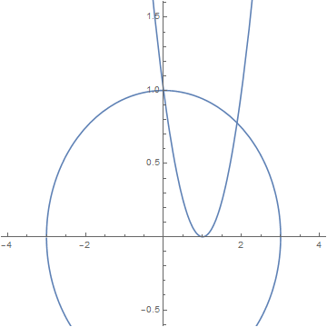
We extend the methods studied previously to the case of systems of nonlinear equations. Let us start with planar case and consider two functions
b = Plot[y /. Solve[x^2 + 9*y^2 - 9 == 0], {x, -4, 4}, AspectRatio -> 1]
Show[a, b, PlotRange -> {-0.5, 1.5}]
Fixed Point Iteration
We consider the problem \( {\bf x} = {\bf g} \left( {\bf x} \right) , \) where \( {\bf g}: \, \mathbb{R}^n \mapsto \mathbb{R}^n \) is the function from n-dimensional space into the same space. The fixed-point iteration is defined by selecting a vector \( {\bf x}_0 \in \mathbb{R}^n \) and defining a sequence \( {\bf x}_{k+1} = {\bf g} \left( {\bf x}_k \right) , \quad k=0,1,2,\ldots . \)
A point \( {\bf x} \in \mathbb{R}^n \) is a fixed point of \( {\bf g} \left( {\bf x} \right) \) if and only if \( {\bf x} = {\bf g} \left( {\bf x} \right) . \) A mapping \( {\bf f} \left( {\bf x} \right) \) is a contractive mapping if there is a positive number L less than 1 such that
Theorem: Let \( {\bf g} \left( {\bf x} \right) \) be a continuous function on \( \Omega = \left\{ {\bf x} = (x_1 , x_2 , \ldots x_n ) \, : \ a_i < x_i < b_i \right\} \) such that
- \( {\bf g} \left( \Omega \right) \subset \Omega ; \)
- \( {\bf g} \left( {\bf x} \right) \) is a contraction.
- g has a fixed point \( {\bf x} \in \Omega \) and the sequence \( {\bf x}_{k+1} = {\bf g} \left( {\bf x}_k \right) , \quad k=0,1,2,\ldots ; \quad {\bf x}_0 \in \Omega \) converges to x;
- \( \| {\bf x}_k - {\bf x} \| \le L^k \,\| {\bf x}_0 - {\bf x} \| . \) ■
Example:
Example. We apply the fixed point iteration to find the roots of the system of nonlinear equations
Do[{x[k + 1] = N[(x[k]^2 - y[k] + 1)/2], y[k + 1] = N[(x[k]^2 + 9*y[k]^2 - 9 + 18*y[k])/18]}, {k, 0, 50}]
Do[Print["i=", i, " x= ", x[i], " y= ", y[i]], {i, 0, 10}]
Do[{y[k + 1] = N[(x[k] - 1)^2], x[k + 1] = N[((x[k] + 1)^2 + 9*y[k]^2 - 10)/2]}, {k, 0, 10}]
Do[Print["i=", i, " x= ", x[i], " y= ", y[i]], {i, 0, 10}]
| k | x_k | y_k | k | x_k | y_k | |
| 0 | 0 | 0.5 | 0 | 0 | 0.5 | |
| 1 | 0.25 | 0.125 | 1 | -3.375 | 1 | |
| 2 | 0.46875 | -0.363715 | 2 | 2.32031 | 19.1406 | |
| 3 | 0.791721 | -0.785364 | 3 | 1649.15 | 1.74323 | |
| 4 | 1.20609 | -0.942142 | 4 | 1.3615*1010 | 2.71639*106 | |
| 5 | 1.6984 | -0.917512 | 5 | 3.41314*1013 | 1.85369*1012 | |
| 6 | 2.40104 | -0.836344 | 6 | 5.97938*1026 | 1.16495*1027 | |
| 7 | 3.80067 | -0.666331 | ||||
| 8 | 8.0557 | -0.141829 | ||||
| 9 | 33.0181 | 2.9734 |
If we use the starting value (1.5, 0.5), then
| k | x_k | y_k | k | x_k | y_k | |
| 0 | 1.5 | 0.5 | 0 | 1.5 | 0.5 | |
| 1 | 1.375 | 0.25 | 1 | -0.75 | 0.25 | |
| 2 | 1.32031 | -0.113715 | 2 | -4.6875 | 3.0625 | |
| 3 | 1.42847 | -0.510404 | 3 | 44.0039 | 32.3477 | |
| 4 | 1.77547 | -0.766785 | 4 | 5716.34 | 1849.34 | |
| 5 | 2.45953 | -0.797679 | 5 | 3.17342056*107 | 3.26652*107 | |
| 6 | 3.92349 | -0.643461 | 6 | 5.3050884*1015 | 1.00706*1015 | |
| 7 | 8.5186 | -0.0812318 | 7 | 1.86357*1031 | 2.8144*1031 | |
| 8 | 36.8239 | 3.45355 | 8 | |||
| 9 | 676.774 | 84.2505 | 9 |
We want to determine why our iterative equations were not suitable for finding the solution near both fixed points (0, 1) and (1.88241, 0.778642). To answer this question, we need to evaluate the Jacobian matrix:
Theorem: Assume that the functions f(x,y) and g(x,y) and their first partial derivatives are continuous in a region that contain the fixed point (p,q). If the starting point is chosen sufficiently close to the fixed point and if
Seidel Method
An improvement analogous to the Gauss-Seiel method for linear systems, of fixe-point iteration can be made. Suppose we try to solve the system of two nonlinear equations
Wegstein Algorithm
Let \( {\bf g} \, : \, \mathbb{R}^n \mapsto \mathbb{R}^n \) be a continuous function. Suppose we are given a system of equations
In planar case, we have two equations
Example:
Example. We apply the Wegstein algorithm to find the roots of the system of nonlinear equations
Newton's Methods
The Newton methods have problems with the initial guess which, in general, has to be selected close to the solution. In order to avoid this problem for scalar equations we combine the bisection and Newton's method. First, we apply the bisection method to obtain a small interval that contains the root and then finish the work using Newton’s iteration.
For systems, it is known the global method called the descent method of which Newton’s iteration is a special case. Newton’s method will be applied once we get close to a root.
Let us consider the system of nonlinear algebraic equations \( {\bf f} \left( {\bf x} \right) =0 , \) where \( {\bf f} \,:\, \mathbb{R}^n \mapsto \mathbb{R}^n , \) and define the scalar multivariable function
- \( \phi ({\bf x}) \ge 0 \) for all \( {\bf x} \in \mathbb{R}^n . \)
- If x is a solution of \( {\bf f} \left( {\bf x} \right) =0 , \) then φ has a local minimum at x.
- At an arbitrary point x0, the vector \( - \nabla \phi ({\bf x}_0 ) \) is the direction of the most rapid decrease of φ.
- φ has infinitely many descent directions.
- A direction u is descent direction for φ at x if and only if \( {\bf u}^T \nabla \phi ({\bf x}) < 0 . \)
- Special descent directions:
(a) Steepest descent method: \( {\bf u}_k = -JF^T ({\bf x}_k )\, {\bf f} ({\bf x}_k ) , \)
(b) Newton’s method: \( {\bf u}_k = -JF^{-1} ({\bf x}_k )\, {\bf f} ({\bf x}_k ) . \) ■
For scalar problems \( f (x) =0 , \) the descent direction is given by \( - \phi' (x) = -2\,f(x) \,f' (x) \) while Newton’s method yields \( -f(x) / f' (x) \) which has the same sign as the steepest descent method.
The question that arises for all descent methods is how far should one go in a given descent direction. To answer this question, there are several techniques and conditions to guarantee convergence to a minimum of φ. For a detailed discussion consult the book by
Numerical Methods for Unconstrained Optimization and Nonlinear Equations, by J. E. Dennis, Jr. and Robert B. Schnabel. Published: 1996, ISBN: 978-0-89871-364-0http://www.math.vt.edu/people/adjerids/homepage/teaching/F09/Math5465/chapter2.pdf
Return to Mathematica page
Return to the main page (APMA0340)
Return to the Part 1 Matrix Algebra
Return to the Part 2 Linear Systems of Ordinary Differential Equations
Return to the Part 3 Non-linear Systems of Ordinary Differential Equations
Return to the Part 4 Numerical Methods
Return to the Part 5 Fourier Series
Return to the Part 6 Partial Differential Equations
Return to the Part 7 Special Functions