Preface


The determinant of a square n×n matrix is calculated as the sum of n! terms, where every other term is negative (i.e. multiplied by -1), and the rest are positive. For the The determinant is a special scalar-valued function defined on the set of square matrices. Although it still has a place in many areas of mathematics and physics, our primary application of determinants is to define eigenvalues and characteristic polynomials for a square matrix A. It is usually denoted as det(A), det A, or |A| and is equal to (-1)n times the constant term in the characteristic polynomial of A. The term determinant was first introduced by the German mathematician Carl Friedrich Gauss in 1801. There are various equivalent ways to define the determinant of a square matrix A, i.e., one with the same number of rows and columns. The determinant of a matrix of arbitrary size can be defined by the Leibniz formula or the Laplace formula.

Return to computing page for the first course APMA0330
Return to computing page for the second course APMA0340
Return to Mathematica tutorial for the first course APMA0330
Return to Mathematica tutorial for the second course APMA0340
Return to the main page for the first course APMA0330
Return to the main page for the second course APMA0340
Return to Part I of the course APMA0340
Introduction to Linear Algebra with Mathematica

Determinants


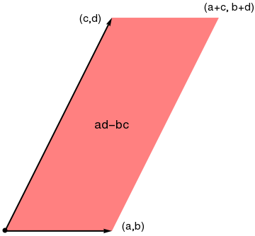
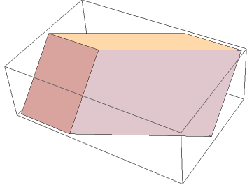
The determinant of a square n×n matrix A is the value that is calculated as the sum of n! terms, half of them are taken with sign plus, and another half has opposite sign. The determinant of a 2×2 matrix is the area of the parallelogram with the column vectors and as two of its sides. Similarly, the determinant of a 3×3 matrix is the volume of the parallelepiped (skew box) with the column vectors, as three of its edges. When the matrix represents a linear transformation, then the determinant (technically the absolute value of the determinant) is the "volume distortion" experienced by a region after being transformed.

The area of the parallelogram
The volume of the parallelepiped
The Leibniz formula for the determinant of an n × n matrix A is
\[ \det\left( {\bf A} \right) = \sum_{\sigma\in S_n} \left( \mbox{sign} (\sigma ) \,\prod_{i=1}^n a_{i, \sigma_i} \right) , \]
where sign is the sign function of permutations in the permutation group Sn, which returns +1 and −1 for even and odd permutations, respectively. Here the sum is computed over all permutations σ of the set {1, 2, …, n}. A permutation is a function that reorders this set of integers. The value in the i-th position after the reordering σ is denoted by σi.

The Laplace expansion, named after Pierre-Simon Laplace, also called cofactor expansion, is an expression for the determinant |A| of an n × n matrix A. It is a weighted sum of the determinants of n sub-matrices of A, each of size (n−1) × (n−1). The Laplace expansion as well as the Leibniz formula, are of theoretical interest as one of several ways to view the determinant, but not for practical use in determinant computation. Therefore, we do not pursue these expansions in detail.

If A is a square matrix, then the minor of the entry in the i-th row and j-th column (also called the (i, j) minor, or a first minor) is the determinant of the submatrix formed by deleting the i-th row and j-th column. This number is often denoted Mi,j. The (i, j) cofactor is obtained by multiplying the minor by (−1)i+j.

If we denote by Cij = (−)i+jMi,j the cofactor of the (i, j) entry of matrix \( {\bf A} = \left[ a_{i,j} \right] , \) then Laplace's expansion can be written as

\begin{equation} \label{EqDet.1} \det ({\bf A}) = a_{1j}C_{1j} + a_{2j}C_{2j} + a_{3j} C_{3j} + \cdots + a_{nj} C_{nj} = \sum_{i=1}^n a_{ij} C_{ij} = \sum_{i=1}^n a_{ij} (-1)^{i+j} {\bf M}_{i,j} \end{equation}
along arbitrary j th column, or
\begin{equation} \label{EqDet.2} \det ({\bf A}) = a_{1j}C_{1,j} + a_{2j}C_{2j} + a_{3j} C_{3j} + \cdots + a_{nj} C_{nj} = \sum_{j=1}^n a_{ij} C_{ij} = \sum_{j=1}^n a_{ij} (-1)^{i+j} {\bf M}_{i,j} \end{equation}
along arbitrary i th row.

The concept of a determinant actually appeared nearly two millennium before its supposed invention by the Japanese mathematician Seki Kowa (1642--1708) in 1683, or his German contemporary Gottfried Leibniz (1646--1716). Traditionally, the determinant of a square matrix is denoted by det(A), det A, or |A|.

In the case of a 2 × 2 matrix (2 rows and 2 columns) A, the determinant is

\[ \det {\bf A} = \det \begin{bmatrix} a&b \\ c&d \end{bmatrix} = \left\vert \begin{array}{cc} a&b \\ c&d \end{array} \right\vert = ad-bc . \]

It is easy to remember when you think of a cross:

  • Blue is positive (\( + ad \) ),
  • Red is negative (\( -bc \) )
  A Matrix

Similarly, for a 3 × 3 matrix (3 rows and 3 columns), we have a specific formula based on the Laplace expansion:
\[ \det \begin{bmatrix} a&b&c \\ d&e&f \\ g&h&i \end{bmatrix} = a\,\left\vert \begin{array}{cc} e&f \\ h&i \end{array} \right\vert - b\,\left\vert \begin{array}{cc} d&f \\ g&i \end{array} \right\vert + c \,\left\vert \begin{array}{cc} d&e \\ g&h \end{array} \right\vert = aei + bfg + cdh - ceg -bdi -afh . \]
Each determinant of a 2 × 2 matrix in this equation is called a "minor" of the matrix A.

It may look complicated, but there is a pattern:

A Matrix

To work out the determinant of a 3×3 matrix:

A similar procedure can be used to find the determinant of a 4 × 4 matrix, the determinant of a 5 × 5 matrix, and so forth, where "minors" are the (n-1) × (n-1) matrices that compose the given n×n matrix.

In Mathematica, the command Det[M] gives the determinant of the square matrix M:

M={{0,1},{-1,3}}; Det[M]
Out[2]= 1

Inverse Matrix


Let \( {\bf A} = \left[ a_{i,j} \right] \) be n×n matrix with cofactors \( C_{ij} = (-1)^{i+j} {\bf M}_{i,j} , \ i,j = 1,2, \ldots , n . \) The matrix formed by all of the cofactors is called the cofactor matrix (also called the matrix of cofactors or, sometimes, comatrix):
\[ {\bf C} = \begin{bmatrix} C_{11} & C_{12} & \cdots & C_{1n} \\ C_{21} & C_{22} & \cdots & C_{2n} \\ \vdots & \vdost & \ddots & \vdots \\ C_{n1} & C_{n2} & \cdots & C_{nn} \end{bmatrix} Then the inverse of A is the transpose of the cofactor matrix times the reciprocal of the determinant of A:
\begin{equation} \label{EqDet.3} {\bf A}^{-1} = \frac{1}{\det ({\bf A})} \, {\bf C}^{\textrm T} . \end{equation} The transpose of the cofactor matrix is called the adjugate matrix of A.
An n × n square matrix A is called invertible if there exists an n × n matrix B such that

\[ {\bf A}\, {\bf B} = {\bf B}\,{\bf A} = {\bf I} , \]
where I is the identity matrix and the multiplication used is ordinary matrix multiplication. If this is the case, then the matrix B is uniquely determined by A and is called the inverse of A, denoted by \( {\bf A}^{-1} . \) If det(A) ≠ 0, then matrix is invertible. A square matrix that is its own inverse, i.e. \( {\bf A} = {\bf A}^{-1} \) and \( {\bf A}^{2} = {\bf I}, \) is called an involution or involutory matrix.

We list the main properties of determinants:

1. \( \det ({\bf I} ) = 1 ,\) where I is the identity matrix (all entries are zeroes except diagonal terms, which all are ones).
2. \( \det \left( {\bf A}^{\mathrm T} \right) = \det \left( {\bf A} \right) . \)
3. \( \det \left( {\bf A}^{-1} \right) = 1/\det \left( {\bf A} \right) = \left( \det {\bf A} \right)^{-1} . \)
4. \( \det \left( {\bf A}\, \ast\, {\bf B} \right) = \det {\bf A} \, \det {\bf B} . \)
5. \( \det \left( c\,{\bf A} \right) = c^n \,\det \left( {\bf A} \right) \) for \( n\times n \) matrix A and a scalar c.
6. If \( {\bf A} = [a_{i,j}] \) is a triangular matrix, i.e. \( a_{i,j} = 0 \) whenever i > j or, alternatively, whenever i < j, then its determinant equals the product of the diagonal entries:

\[ \det \left( {\bf A} \right) = a_{1,1} a_{2,2} \cdots a_{n,n} = \prod_{i=1}^n a_{i,i} . \]
The adjugate of a square matrix is the transpose of its cofactor matrix.
Example 1: Consider the 3×3 matrix
\[ {\bf A} = \begin{bmatrix} 1&\phantom{-}4&3 \\ 2&-1&2 \\ 1&\phantom{-}2&2 \end{bmatrix} \]
First, we check whether the matrix is not singular:
A = {{1, 4, 3}, {2, -1, 2}, {1, 2, 2}}; Det[A]
1
Then we use Mathematica to find its inverse
Inverse[A]
{{-6, -2, 11}, {-2, -1, 4}, {5, 2, -9}}
\[ {\bf A}^{-1} = \begin{bmatrix} 1&\phantom{-}4&3 \\ 2&-1&2 \\ 1&\phantom{-}2&2 \end{bmatrix}^{-1} = \begin{bmatrix} -6&-2&11 \\ -2&-1&\phantom{-}4 \\ \phantom{-}5& \phantom{-}2&-9 \end{bmatrix} . \]
Now we find its inverse manually. First, we calculate the minor matrix:
\[ {\bf M} = \begin{bmatrix} -6& \phantom{-}2& \phantom{-}5 \\ \phantom{-}2& -1&-2 \\ 11 & -4& -9 \end{bmatrix} \]
because
\[ m_{11} = \begin{bmatrix} -1&2 \\ 2&2 \end{bmatrix} = -6, \quad m_{12} = \begin{bmatrix} 2&2 \\ 1&2 \end{bmatrix} =2, \quad m_{13} = \begin{bmatrix} 2&-1 \\ 1&2 \end{bmatrix} = 5, \quad m_{21} = \begin{bmatrix} 4&3 \\ 2&2 \end{bmatrix} = 2, \]
and so on. Since the determinant of matrix A is 1, its inverse is just transposed matrix M, each element being multiplied by either 1 or −1.    ▣
Example 2: Consider the 2×2 matrix
\[ {\bf B} = \begin{bmatrix} \phantom{-}0&1 \\ -1&0 \end{bmatrix} , \]
which we enter into Mathematica notebook as
B := {{0, 1}, {-1, 0}}
Out[1]= {{0, 1}, {-1, 0}}
Its inverse is \( {\bf B}^{-1} = -{\bf B} = \begin{bmatrix} 0&-1 \\ 1&\phantom{-}0 \end{bmatrix} . \)
Inverse[B]
Out[2]= {{0, -1}, {1, 0}}
Its second power \( {\bf B}\,{\bf B} = {\bf B}^2 = - \begin{bmatrix} 1 & 0 \\ 0 & 1 \end{bmatrix} = -{\bf I} = \begin{bmatrix} -1 & \phantom{-}0 \\ \phantom{-}0 & -1 \end{bmatrix} \) is the negative identity matrix. Next, we calculate its third power \( {\bf B}\,{\bf B}\,{\bf B} = {\bf B}^3 = - {\bf B} , \) and finally the fourth power of the matrix B, which is the identity matrix: \( {\bf B}^4 = {\bf I} . \)
B.B.B.B
Out[3]= {{1, 0}, {0, 1}}
   ▣
A matrix A is called singular if and only if its determinant is zero. Otherwise, the matrix is nonsingular or invertible (because an inverse matrix exists for such matrix).
The Cayley--Hamilton method for a 2 × 2 matrix gives
\[ {\bf A}^{-1} = \frac{1}{\det {\bf A}} \left[ \left( \mbox{tr} {\bf A} \right) {\bf I} - {\bf A} \right] . \]

We list some basic properties of the inverse operation:

1. \( \left( {\bf A}^{-1} \right)^{-1} = {\bf A} . \)
2. \( \left( c\,{\bf A} \right)^{-1} = c^{-1} \,{\bf A}^{-1} \) for nonzero scalar c.
3. \( \left( {\bf A}^{\mathrm T} \right)^{-1} = \left( {\bf A}^{-1} \right)^{\mathrm T} . \)
4. \( \left( {\bf A}\, {\bf B} \right)^{-1} = {\bf B}^{-1} {\bf A}^{-1} . \)

Theorem: For a square matrix A, the homogeneous equation Ax = 0 has a nontrivial solution (meaning not zero) if and only if the matrix A is singular, so its determinant must be zero.
If A is an invertible square matrix (its determinant is not zero), then we can multiply both sides of the equation Ax = 0 by the inverse matrix A−1 to obtain
\[ {\bf A}^{-1} {\bf A}\,{\bf x} = {\bf x} = {\bf A}^{-1} {\bf 0} \qquad \Longrightarrow \qquad {\bf x} = {\bf 0} . \]
A square matrix whose transpose is equal to its inverse is called an orthogonal matrix; that is, A is orthogonal if \( {\bf A}^{\mathrm T} = {\bf A}^{-1} . \)
Example 3: In three-dimensional space, consider the rotational matrix
\[ {\bf A} = \begin{bmatrix} \cos\theta & 0& -\sin\theta \\ 0&1& 0 \\ \sin\theta & 0& \phantom{-}\cos\theta \end{bmatrix} , \]
where θ is any angle. This matrix describes a rotation in the (x1, x3) plane in ℝ³. WE ch3eck its properties with Mathematica:
A = {{Cos[theta], 0,-Sin[theta]}, {0,1,0},{Sin[theta],0,Cos[theta]}};
Simplify[Inverse[A]]
{{Cos[theta], 0, Sin[theta]}, {0, 1, 0}, {-Sin[theta], 0, Cos[theta]}}
Simplify[Transpose[A] - Inverse[A]]
{{0, 0, 0}, {0, 0, 0}, {0, 0, 0}}
\[ {\bf A}^{-1} = {\bf A}^{\textrm T} = \begin{bmatrix} \phantom{-}\cos\theta & 0& \sin\theta \\ 0&1& 0 \\ -\sin\theta & 0 & \cos\theta \end{bmatrix} , \]


For any unit vector v, we define the reflection matrix:
\[ {\bf R} = {\bf I} - 2 {\bf v}\,{\bf v}^{\textrm T} . \]
Upon choosing v = [1, 2, −2]/3, we get
\[ {\bf v}\,{\bf v}^{\textrm T} = \frac{1}{9} \begin{bmatrix} \phantom{-}1& \phantom{-}2&-2 \\ \phantom{-}2& \phantom{-}4 &-4 \\ -2&-2& 4 \end{bmatrix} \qquad \Longrightarrow \qquad {\bf R} = \frac{1}{9} \begin{bmatrix} \phantom{-}7&-4&4 \\ -4&\phantom{-}1& 8 \\ \phantom{-}4&\phantom{-}8& 1 \end{bmatrix} . \]
Its inverse is
\[ {\bf R}^{-1} = {\bf R}^{\textrm T} = \frac{1}{9} \begin{bmatrix} \phantom{-}7& -4& \phantom{-}4 \\ -4& \phantom{-}1 &\phantom{-}8 \\ \phantom{-}4& \phantom{-}8& \phantom{-}1 \end{bmatrix} . \]
R = {{7, -4, 4}, {-4, 1, 8}, {4, 8, 1}}/9 ;
Inverse[R]
{{7/9, -(4/9), 4/9}, {-(4/9), 1/9, 8/9}, {4/9, 8/9, 1/9}}
Inverse[R] - Transpose[R]
{{0, 0, 0}, {0, 0, 0}, {0, 0, 0}}
   ■


  1. Bibliography for the Inverse Matrix
  2. Axler, S., Linear Algebra Done Right, Springer; NY, 2014.
  3. Hannah, John, A geometrical approach to determinants, The American mathematical Monthly, 1996, Vol. 103, No. 5, pp. 401--409.
  4. Yandl, A.L. and Swenson, C., A class of matrices with zero determinant, Mathematics Magazine, 2012, Vol. 85, Issue 2, pp. 126--130. https://doi.org/10.4169/math.mag.85.2.126


Return to Mathematica page
Return to the main page (APMA0340)
Return to the Part 1 Matrix Algebra
Return to the Part 2 Linear Systems of Ordinary Differential Equations
Return to the Part 3 Non-linear Systems of Ordinary Differential Equations
Return to the Part 4 Numerical Methods
Return to the Part 5 Fourier Series
Return to the Part 6 Partial Differential Equations
Return to the Part 7 Special Functions