Example:
Consider the matrix
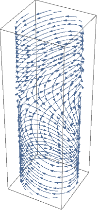
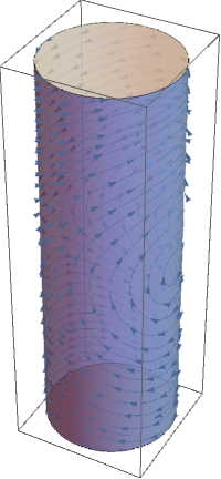
You can draw phase portrait for the pendulum not on the plane
\( \mathbb{R}^2 , \) but
on the cylinder
\( S^1 \times \mathbb{R} . \) The pendulum of course has only two
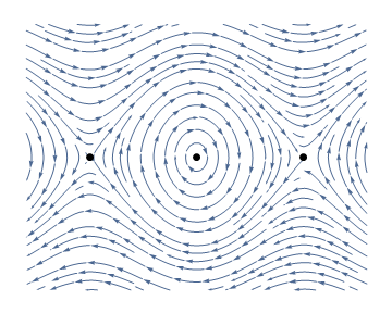
equilibria, one at (0,0) and another one at (π,0).
plot = StreamPlot[{y, -Sin[x]}, {x, -Pi, Pi}, {y, -3, 3}, Frame -> None,
Epilog -> {PointSize -> Large, Point[{{0, 0}, {π, 0}, {-π, 0}}]},
StreamPoints -> Fine, AspectRatio -> 0.8]
First[Normal@plot] /. a_Arrow :> (
a /. {x_Real, y_Real} :> {Cos[x], Sin[x], y}
) // Graphics3D
Show[ %,
Graphics3D@{Opacity@.7, LightBlue, Cylinder[{{0, 0, -3}, {0, 0, 3}}]}
]
img = Image@StreamPlot[{y, -Sin[x]}, {x, -5, 5}, {y, -3, 3},
Frame -> None,
PlotRange -> {{-5, 5}, {-3, 3}},
Epilog -> {PointSize -> Large,
Point[{{0, 0}, {Pi, 0}, {-Pi, 0}}]}, StreamPoints -> Fine,
AspectRatio -> 0.8, PlotRangePadding -> 0, ImageMargins -> 0,
ImageSize -> 800];
Graphics3D[{Texture[img], EdgeForm[],
cyl[{{0, 0, 0}, {0, 0, 2 Pi}}, 1]}, Boxed -> False]
img = Rasterize[
StreamPlot[{y, -Sin[x]}, {x, -5, 5}, {y, -3, 3}, Frame -> None,
PlotRange -> {{-5, 5}, {-3, 3}},
Epilog -> {PointSize -> Large,
Point[{{0, 0}, {Pi, 0}, {-Pi, 0}}]}, StreamPoints -> Fine,
AspectRatio -> 0.8, PlotRangePadding -> 0, ImageMargins -> 0,
ImageSize -> 500], Background -> None, ImageResolution -> 300];
Graphics3D[{Texture[ImageData@img], EdgeForm[],
Cylinder[{{0, 0, 0}, {0, 0, 2 Pi}}, 1]}, Boxed -> False,
Lighting -> "Neutral"]
The vector field can also be interpreted as a velocity vector field. This means that a point
in the phase space moves along a trajectory so that its velocity vector at each instant equals the vector of the vector field attached to the location of
. Such a trajectory X(t), also called an orbit, trajectory, streamline, is simply the solution of an ordinary differential equation
It is however more convenient to represent the trajectories on a plane instead of on a cylinder. This can be done by expanding the cylindrical phase space by periodicity onto a phase plane. The following diagram is called a phase portrait.
StreamPlot[{y, -Sin[x]}, {x, -5, 5}, {y, -3, 3},
Frame -> None, StreamPoints -> Fine, AspectRatio -> 0.8,
Epilog -> {PointSize -> Large, Point[{{0, 0}, {\[Pi], 0}, {-\[Pi], 0}}]}]
\[
\dot{\bf x} = {\bf f}({\bf x}) =0 \qquad \Longrightarrow \qquad \begin{cases} y&=0 , \\ \sin x &=0 . \end{cases}
\]
\[
\begin{cases} y&=0 , \\ x &=n\pi , \quad \mbox{with $n$ integer} . \end{cases}
\]