Preface


This section presents some applications of Fourier transformation in heat transfer problems for unbounded domains.

Return to computing page for the first course APMA0330
Return to computing page for the second course APMA0340
Return to Mathematica tutorial for the first course APMA0330
Return to Mathematica tutorial for the second course APMA0340
Return to the main page for the first course APMA0330
Return to the main page for the second course APMA0340
Return to Part VI of the course APMA0340
Introduction to Linear Algebra

Blasius equation


A Blasius boundary layer (named after the German fluid dynamics physicist Paul Richard Heinrich Blasius, 1883--1970) describes the steady two-dimensional laminar boundary layer that forms on a semi-infinite plate which is held parallel to a constant unidirectional flow. Upon introducing a normalized stream function f, the Blasius equation becomes
\[ f''' + \frac{1}{2}\,f\,f'' =0 . \]
The boundary conditions are the no-slip condition:
\[ f(0) =0 , \qquad f' (0) =0, \qquad \lim_{y\to\infty} f' (y) = 0 . \]
This is a nonlinear, boundary value problem (BVP) for the third order differential equation. The main obstacle in solving this problem numerically is request to evaluate f'(∞). Several strategies have been proposed in order to bypass this evaluation. One of them is to convert the given problem into the initial value problem, which was first achieved by K. Töpfer in 1912 by constructing a transformation of variables that reduces the BVP into an IVP. Actually, this leads to determination of the second derivative at the origin, f''(0), called the Blasius constant. Its numerical value was obtained by many researchers starting with K. Töpfer; however, the rigorous derivation of the Blasius constant is due to V.P. Varin in 2013 who obtained it in the form of a convergent series of rational numbers. Therefore, we assume that its value a = f′′(0) ≈ 0.33205733621 to be known (which is slightly less than 1/3). The knowledge of the Blasius constant is also necessary to evaluate the shear stress at the plate. Once this value is determined, we obtain the initial value problem, which can be solved numerically. So we solve the relevant initial value problem using different methods.

First, we start with Picard's iteration, and to achieve this we have two options: either to apply Picard's iteration directly to the third order Blasius equation directly or to convert it to a system of first-order differential equations. So we demonstrate both options, beginning with the latter.
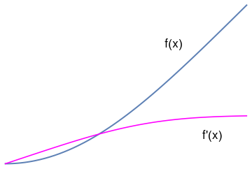
blasius = NDSolve[{f'''[x] + 1/2*f[x]*f''[x] == 0, f[0] == 0, f'[0] == 0, f''[0] == 1/3}, f, {x, 0, 5}]
g = Plot[Evaluate[{f[x], f'[x]} /. blasius], {x, 0, 5}, PlotStyle -> {Thick, {Blue, Magenta}}]
txt1 = Graphics[ Text[Style["f(x)", FontSize -> 16, Black], {3.5, 2.5}]]
txt2 = Graphics[ Text[Style["f'(x)", FontSize -> 16, Black], {4.3, 0.6}]]
Show[txt1, txt2, g]


Classical Picard's iteration

In order to apply the classical Picard's iteration, we have to convert this to a system of first-order differential equations. Let

\[ f_1 = f, \qquad f_2 = f' , \qquad\mbox{and} \qquad f_3 = f'' . \]
This leads to:
\[ \frac{\text d}{{\text d}y} \begin{bmatrix} f_1 \\ f_2 \\ f_3 \end{bmatrix} = \begin{bmatrix} f_2 \\ f_3 \\ - \frac{1}{2}\, f_1 f_3 \end{bmatrix}, \qquad f_1 (0) =0, \quad f_2 (0) =0, \quad f_2 (\infty ) =1. \]
It is not possible to specify a boundary condition at ∞ numerically, so we will have to use a large number, and verify it is "large enough". From the solution, we evaluate the derivatives at y = 0, and we have f''(0) = f3(0).

We have to provide initial guesses for f1, f2 and f3. This is the hardest part about this problem. We know that f1 starts at zero, and is flat there (f'(0)=0), but at large y, it has a constant slope of one. We will guess a simple line of slope = 1 for f1. That is correct at large y, and is zero at y = 0. If the slope of the function is constant at large y, then the values of higher derivatives must tend to zero. We choose an exponential decay as a guess.

Finally, we let a solver iteratively find a solution for us, and find the answer we want. The solver is in the pycse module.


import numpy as np
from pycse import bvp

def odefun(F, x):
    f1, f2, f3 = F.T
    return np.column_stack([f2,
                            f3,
                            -0.5 * f1 * f3])

def bcfun(Y):
    fa, fb = Y[0, :], Y[-1, :]
    return [fa[0],        # f1(0) =  0
            fa[1],        # f2(0) = 0
            1.0 - fb[1]]  # f2(inf) = 1

eta = np.linspace(0, 6, 100)
f1init = eta
f2init = np.exp(-eta)
f3init = np.exp(-eta)

Finit = np.column_stack([f1init, f2init, f3init])

sol = bvp(odefun, bcfun, eta, Finit)
f1, f2, f3 = sol.T

print("f''(0) = f_3(0) = {0}".format(f3[0]))

import matplotlib.pyplot as plt
plt.plot(eta, f1)
plt.xlabel('$\eta$')
plt.ylabel('$f(\eta)$')
plt.savefig('images/blasius.png')

We get the initial second derivative to be f''(0) = 0.3324911095517483. For the sake of simplicity, we approximate the Blasius constant as 1/3.

Now we use Picard iteration procedure starting with the initial conditions. Since the derivative operator is unbounded, we apply its inverse to reduce the given initial value problem into fixed point form:

\[ \frac{\text d}{{\text d}y} \begin{bmatrix} f_1 \\ f_2 \\ f_3 \end{bmatrix} = \begin{bmatrix} f_2 \\ f_3 \\ - \frac{1}{2}\, f_1 f_3 \end{bmatrix}, \qquad \begin{bmatrix} f_1 (0) \\ f_2 (0) \\ f_3 (0) \end{bmatrix} = \begin{bmatrix} 0 \\ 0 \\ 1/3 \end{bmatrix} \qquad \Longleftrightarrow \qquad \begin{bmatrix} f_1 (y) \\ f_2 (y) \\ f_3 (y)\end{bmatrix} = \begin{bmatrix} f_1 (0) \\ f_2 (0) \\ f_3 (0) \end{bmatrix} + \int_0^y \begin{bmatrix} f_2 (s) \\ f_3 (s) \\ - \frac{1}{2}\, f_1 (s)\,f_3 (s) \end{bmatrix} {\text d}s . \]
From this fixed point equation, we derive the iteration procedure
\[ \begin{bmatrix} f_{1,n+1} (y) \\ f_{2,n+1} (y) \\ f_{3,n+1} (y) \end{bmatrix} = \begin{bmatrix} 0 \\ 0 \\ 1/3 \end{bmatrix} + \int_0^y \begin{bmatrix} f_{2,n} (s) \\ f_{3, n} (s) \\ - \frac{1}{2}\, f_{1,n} (s)\,f_{3,n} (s) \end{bmatrix} {\text d}s , \qquad n=0,1,2,\ldots . \]
The initial approximation is just the initial conditions:
\[ \phi_{1,0} =0, \quad \phi_{2,0} =0, \quad \phi_{3,0} = 1/3 \quad\mbox{however, it should be the Blasius constant}. \]
The first iteration becomes
\[ \begin{bmatrix} \phi_{1,1} (y) \\ \phi_{2,1} (y) \\ \phi_{3,1} (y) \end{bmatrix} = \begin{bmatrix} 0 \\ 0 \\ 1/3 \end{bmatrix} + \int_0^y \begin{bmatrix} 0 \\ 1/3 \\ 0 \end{bmatrix} {\text d} y = \begin{bmatrix} 0 \\ y/3 \\ 1/3 \end{bmatrix} . \]
The second one is
\[ \begin{bmatrix} \phi_{1,2} (y) \\ \phi_{2,2} (y) \\ \phi_{3,2} (y) \end{bmatrix} = \begin{bmatrix} 0 \\ 0 \\ 1/3 \end{bmatrix} + \int_0^y \begin{bmatrix} y/3 \\ 1/3 \\ 0 \end{bmatrix} {\text d} y = \begin{bmatrix} y^2 /6 \\ y/3 \\ 1/3 \end{bmatrix} = \frac{1}{3} \begin{bmatrix} y^2 /2 \\ y \\ 1 \end{bmatrix} . \]
The third one is
\[ \begin{bmatrix} \phi_{1,3} (y) \\ \phi_{2,3} (y) \\ \phi_{3,3} (y) \end{bmatrix} = \begin{bmatrix} 0 \\ 0 \\ 1/3 \end{bmatrix} + \int_0^y \begin{bmatrix} y/3 \\ 1/3 \\ - y^2/36 \end{bmatrix} {\text d} y = \begin{bmatrix} y^2 /6 \\ y/3 \\ 1/3 - y^3/108 \end{bmatrix} = \frac{1}{3} \begin{bmatrix} y^2 /2 \\ y \\ 1 - y^3/36 \end{bmatrix} . \]
For next one, we have
\[ \begin{bmatrix} \phi_{1,4} (y) \\ \phi_{2,4} (y) \\ \phi_{3,4} (y) \end{bmatrix} = \begin{bmatrix} 0 \\ 0 \\ 1/3 \end{bmatrix} + \int_0^y \begin{bmatrix} y/3 \\ 1/3 - y^3/108 \\ - \frac{1}{36} \left( y^2 - \frac{y^5}{36} \right) \end{bmatrix} {\text d} y = \begin{bmatrix} y^2 /6 \\ \frac{y}{3} - \frac{y^4}{4 \cdot 108} \\ \frac{y^6}{36^3 \cdot 6} - \frac{y^3}{6\cdot 26} \end{bmatrix} = \frac{1}{3} \begin{bmatrix} y^2 /2 \\ y - \frac{y^4}{4 \cdot 36} \\ \frac{y^6}{2\cdot 36^2} - \frac{y^3}{36} \end{bmatrix} . \]
So ur fifth approximation becomes
f1[y_] = y^2/6; f2[y_] = 1/3*(y - y^4/4/36); f3[y_] = 1/3*(y^6/2/36^2 - y^3 /36); f5[y_] = Simplify[Integrate[1/9*(s - s^4 /4/36), {s, 0, y}]]
-((y^2 (-360 + y^3))/6480)
\[ f_5 (y) = \frac{y^2}{6480} \left( 360 - y^3 \right) . \]


Picard's iteration applied to the third order equation

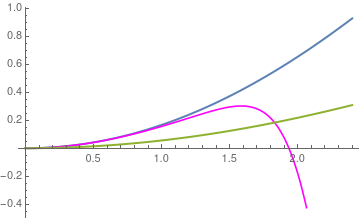
We use the fixed point formulation of the given initial value problem:

\[ f(x) = \frac{1}{6} - \frac{1}{4} \int_0^x \left( x-s \right)^2 f(s)\,f''(s) \,{\text d}s . \]
This leads to the following iteration procedure:
\[ y_{n+1} (x) = \frac{x^2}{6} - \frac{1}{4} \int_0^x \left( x-s \right)^2 y_n (s) \,y_{n}''(s) \,{\text d}s , \qquad n=3,4,\ldots , \]
with the following initial values:
\[ y_0 = 0, \quad y_1 =0, \quad y_2 = \frac{x^2}{6} . \]
For simplicity, we employ the Blasius constant to be 1/3. Next iteration results
y2[x_] = x^2 /6
y3[x_] = Simplify[ y2[x] - 1/4*Integrate[(x - s)^2*y2[x]*1/3, {s, 0, x}]]
-(1/216) x^2 (-36 + x^3)
\[ y_3 (x) = \frac{x^2}{216} \left( 36 - x^3 \right) . \]
We proceed with Mathematica.
y4[x_] = Simplify[ y3[x] - 1/4*Integrate[(x - s)^2*y2[x]*D[y3[x], x, x], {s, 0, x}]]
(x^2 (23328 - 1296 x^3 + 198 x^6 - 5 x^9))/139968
y5[x_] = Simplify[ y4[x] - 1/4*Integrate[(x - s)^2*y4[x]*D[y4[x], x, x], {s, 0, x}]]
\[ f_5 (x) = \frac{x^2}{117546246144} \left( 19591041024 - 1632586752 x^3 + 498845952 x^6 - 154944576 x^9 + 16282944 x^{12} - 1518912 x^{15} + 82170 x^{18} - 1375 x^{21} \right) . \]
Now we plot the fifth approximation along with the numerical solution obtained by Mathematica.
Plot[{Evaluate[{f[x]} /. blasius], y5[x], f5[x]}, {x, 0, 2.4}, PlotStyle -> {Thick, {Blue, Orange, Magenta}}]
Therefore, we see that the two Picard's iteration procedures do not coincide and provide two different approximations. Moreover, the Picard's iteration applied directly to the third order equation converges much faster than the iteration based on reduction to the first order system of equations.


Power Series Method


Adomian Decomposition Method

text goes here


  1. Aminikhah, Hossein, Analytical Approximation to the Solution of Nonlinear Blasius’ Viscous Flow Equation by LTNHPM, ISRN Mathematical Analysis Volume 2012, Article ID 957473, 10 pages http://dx.doi.org/10.5402/2012/957473
  2. Blasius, H., Grenzschichten in Flüssigkeiten mitkleiner Reibung, Zeitschrift für angewandte Mathematik und Physik (Journal of Applied Mathematics and Physics), 56:137, 1908.
  3. Solving the Blasius equation
  4. The Blasius equation, B. Bright, A. Fruchard, and T. Sari, 2010.
  5. Blasius equation
  6. Fazio, R., Transformation methods for the Blasius problem and its recent variants, Proceedings of the World Congress on Engineering, 2008 Vol IIWCE 2008, July 2 - 4, 2008, London, U.K.
  7. Mattioli, Franco, Blasius solution, University of Bologna, Italy.
  8. Parand, K., Dehghan, M., and Taghavi, A., Modified generalized Laguerre function Tau method for solving laminar viscous flow: The Blasius equation, Journal of Numerical methods for Heat & Fluid Flow, 2010, Vol. 20, Issue 7, pp.728--743, https://doi.org/10.1108/09615531011065539
  9. Puttkammer, P.P., Boundary Layer over a Flat Plate, University of Twenter, 2013.
  10. Töpfer, K., Bemerkung zu dem Aufsatz von H. Blasius: Grenzschichten in Flüssigkeiten mit kleinerReibung, Zeitschrift für angewandte Mathematik und Physik (Journal of Applied Mathematics and Physics), 60:397–398, 1912
  11. Treve, Y.M., On a class of solutions of the Blasius equation with applications, SIAM Journal of Applied Mathematics, 1967, Vol. 15, No. 5, 1209--1227. doi: 10.1137/0115103
  12. Varin, V.P., A solution of the Blasius problem, Keldysh Institute, Preprint No. 40, 2013.
  13. Weidman, P.D., Blasius boundary layer flow over an irregular leading edge, Physics of Fluids, 9, 1470 (1997); https://doi.org/10.1063/1.869268
  14. Zheng, J., Han, X., Wang, Z., Li, C., and Zhang, J., A globally convergent and closed analytical solution of the Blasius equation with beneficial applications, AIP Advances, Vol. 7, 065311 (2017); https://doi.org/10.1063/1.4985741


Return to Mathematica page
Return to the main page (APMA0340)
Return to the Part 1 Matrix Algebra
Return to the Part 2 Linear Systems of Ordinary Differential Equations
Return to the Part 3 Non-linear Systems of Ordinary Differential Equations
Return to the Part 4 Numerical Methods
Return to the Part 5 Fourier Series
Return to the Part 6 Partial Differential Equations
Return to the Part 7 Special Functions