Return to
computing page for the first course APMA0330
Return to
computing page for the second course APMA0340
Return to
Mathematica tutorial for the first course APMA0330
Return to
Mathematica tutorial for the second course APMA0340
Return to the
main page for the
first course APMA0330
Return to the
main page for the
second course APMA0340
Return to
Part VI of the course APMA0340
Introduction to
Linear Algebra
This section gives an introduction to the Fourier transformation and presents some applications to heat
transfer problems for unbounded domains. Since the Fourier transform of a function f (x ), x ∈ℝ, is an indefinite integral \eqref{EqFourier.1} containing high-oscillation multiple, its numerical evaluation is an ill-posed problem. For its regularization, as well as for its inverse, it is a custom to define it as the Cauchy principle value .
There are several common conventions for defining the
Fourier transform of an integrable
complex-valued function f : ℝ → ℂ. We use the following notation for the Fourier transformation and its inverse.
\begin{equation} \label{EqFourier.1}
\hat{f} (\xi ) = ℱ\left[ f(x) \right] (\xi ) = f^F (\xi ) =
\int_{-\infty}^{\infty} f(t)\,e^{{\bf j} \xi\cdot t} \,{\text d}t = \lim_{N\to\infty} \int_{-N}^N f(t)\,e^{{\bf j} \xi\cdot t} \,{\text d}t ,
\end{equation}
with the inverse (that is valid for functions satisfying the
Dirichlet conditions )
\begin{equation} \label{EqFourier.2}
f(t) = ℱ^{-1} \left( \hat{f} \right) =
\text{V.P.} \frac{1}{2\pi} \int_{-\infty}^{\infty} \hat{f}(\xi )\,e^{-{\bf j}
\xi\cdot t} \,{\text d}\xi = \lim_{N\to \infty} \frac{1}{2\pi} \int_{-N}^N
\hat{f}(\xi )\,e^{-{\bf j}
\xi\cdot t} \,{\text d}\xi = \frac{f(t+0) + f(t-0)}{2} .
\end{equation}
Since integration is not sensitive for changing the values of integrand at discrete number of points, Fourier transform may assign the same value to many functions. In order to maintain uniqueness of Fourier transform, mathematicians identify all functions having the same Fourier transform into one element, which is also called a function. This requies utilization of Lebesque integration rather than Riemann integration , studied in calculus. Our objective is to use some properties of Fourier transformion, but to expose this topic, which is a part of harmonic analysis .
A treatment of Fourier transformion is impossible without introducing two function spaces. The first of them, denoted by 𝔏¹(ℝ) or simpley 𝔏¹ consists of all Lebesgue integrable functions:
\[
\int_{-\infty}^{\infty} \left\vert f(x) \right\vert {\text d} x < \infty \qquad \Longrightarrow \qquad f \in 𝔏^{1}(\mathbb{R}) .
\]
Another important space constitute square integrable function:
\[
\int_{-\infty}^{\infty} \left\vert f(x) \right\vert^2 {\text d} x < \infty \qquad \Longrightarrow \qquad f \in 𝔏^{2}(\mathbb{R}) .
\]
Fourier transformion exists for functions from both spaces, 𝔏¹(ℝ) and 𝔏²(ℝ); however, there is known a function
f (
x ) for which its Fourier transform exists, but
f (
x ) is not integrable. It is known that the Fourier transform ℱ maps 𝔏²(ℝ) → 𝔏²(ℝ) as an (isometric)
isomorphism and 𝔏¹(ℝ) → 𝔏
∞ (ℝ) as a bounded operator. Out of many properties (see
section of Part V) of the Fourier transformion, we indicate the most important one related to our ropic: it gives a spectral representation of the derivative operator:
\begin{equation} \label{EqFourier.3}
ℱ_{x\to \xi} \left[ \frac{{\text d}f}{{\text d}x} \right] = -{\bf j}\xi ℱ\left[ f(x) \right] (\xi ) = -{\bf j}\xi \,\hat{f}(\xi ) .
\end{equation}
Riemann–Lebesgue lemma:
If
ƒ ∈ 𝔏¹(ℝ) is absolutely integrable, then the Fourier transform of
ƒ satisfies
\[
\hat{f}(\xi ) = \mbox{P.V.}\,\int_{-\infty}^{\infty} f(x)\, e^{{\bf j}\xi x} {\text d}x \ \to \ 0 \qquad\mbox{as} \quad \xi \ \to\ \infty .
\]
Theorem 2:
If
ƒ (
z ) is an analytic function in the upper complex plane Im
z ≥ 0 except points
z 1 ,
z 2 , … ,
z n with positive imaginary parts, and if
\[
\lim_{R\to\infty} \left[ \mas_{|z|=R, \ \Im z > 0} \left\vert f(z) \right\vert \right] = 0 ,
\]
then for ξ > 0
\[
\mbox{P.V.}\,\int_{-\infty}^{\infty} f(x)\, e^{{\bf j}\xi x} {\text d}x = 2\pi {\bf j} \sum_{i=1}^n \mbox{Res}_{z_i} \left[ f(z)\,e^{{\bf j}\xi z} \right] .
\]
Example 1: Some examples of Fourier transforms
Example 1:
\[
f(x) - \frac{x}{1+x^2} \in 𝔏²(\mathbb{R}), \qquad\mbox{but} \quad f(x) \not\in 𝔏¹(\mathbb{R}).
\]
For ξ > 0, we apply Theorem 2:
\[
\hat{f} (\xi ) = \mbox{P.V.} \int_{-\infty}^{\infty} f(x)\, e^{{\bf j} x \xi} {\text d}x = 2\pi{\bf j} \,\mbox{Res}_{z={\bf j}} \,\frac{z}{1 + z^2}\, e^{{\bf j} z \xi} = \pi {\bf j}\, e^{-\xi} , \qquad \xi > 0.
\]
For ξ < 0, we have
\[
\hat{f} (\xi ) = \mbox{P.V.} \int_{-\infty}^{\infty} f(x)\, e^{{\bf j} x \xi} {\text d}x = 2\pi{\bf j} \,\mbox{Res}_{z= -{\bf j}} \,\frac{z}{1 + z^2}\, e^{{\bf j} z \xi} = -\pi {\bf j}\, e^{\xi} , \qquad \xi < 0.
\]
■
Example 2: 𝔏¹(ℝ) and 𝔏²(ℝ) are distinct spaces
Example 2:
\[
f(x) = \frac{1}{\sqrt{x} \left( 1 + x^2 \right)} \in 𝔏^{1}(\mathbb{R}) .
\]
However, this function is not square integrable. On the other hand,
\[
g(x) = \frac{x}{1 + x^2} \in 𝔏^{2}(\mathbb{R}) .
\]
However, this function is not integrable.
■
We start with the easiest problem for the diffusion equation---the initial
value problem for an infinite rod:
\[
\begin{split}
u_t &= \alpha\, u_{xx} , \qquad x \in (-\infty ,\infty ), \quad t > 0,
\\
u(x,0) &= f(x) ,
\end{split}
\]
where the thermal diffusivity α is assumed to be a positive constant. It is also assumed that the solution and its derivatives are square integrable, so they belong to the space 𝔏².
We can solve this problem with Mathematica :
Clear[All]
Integrate[(E^(-((x - K[1])^2/(4 aa t))) f[K[1]])/(
2 Sqrt[\[Pi]] Sqrt[aa t]), {K[1], -\[Infinity], \[Infinity]},
Assumptions -> aa > 0 && t > 0 && {aa, t} > 0]
To solve the given initial value problem, we apply the exponential Fourier transformation. So we multiply both sides of the heat equation by the exponential function
\( e^{{\bf j} kx} \) and integrate with respect to
x to obtain
\[
\int_{-\infty}^{\infty} \frac{\partial u}{\partial t}\,e^{{\bf j} kx}\, {\text d}x = \alpha \int_{-\infty}^{\infty} \frac{\partial^2 u}{\partial x^2}\,e^{{\bf j} kx}\, {\text d}x .
\]
It is assumed that all integrals exist, so partial derivatives of
u (
x, t ) decay fast at infinity. Therefore, we can integrate by parts the latter integral and exchange the order of differentiation with respect to
t and integration with respect to
x in the former integral, This yields
\[
\frac{\text d}{{\text d}t} \int_{-\infty}^{\infty} u(x,t)\,e^{{\bf j} kx}\, {\text d}x = - k^2 \int_{-\infty}^{\infty} u(x,t)\,e^{{\bf j} kx}\, {\text d}x .
\]
Using notation
\[
u^F (k,t) = ℱ\left[ u(x,t) \right] = \int_{-\infty}^{\infty} u(x,t)\,e^{{\bf j} kx}\, {\text d}x ,
\]
we get the initial value problem for the Fourier transform of the unknown function
u (
x, t ):
\[
\frac{\text d}{{\text d}t} \,u^F (k,t) + \alpha\,k^2 ,u^F (k,t) = 0, \qquad ,u^F (k,0) = f^F (k) = \int_{-\infty}^{\infty} f(x)\,e^{{\bf j} kx}\, {\text d}x .
\]
Since the governed equation is linear, we find its solution
Assuming[ A > 0, DSolve[{v'[t] + A*v[t] == 0, v[0] == fF}, v, t]]
{{v -> Function[{t}, E^(-A t) fF]}}
\[
u^F (k,t) = f^F (k)\,e^{-\alpha\,k^2 t} .
\]
Now applying the inverse Fourier transform, we obtain the required solutions in terms of Fourier integral:
\[
u(x,t) = ℱ^{-1} \left[ u^F (k,t) \right] = \frac{1}{2\pi} \int_{-\infty}^{\infty} e^{-{\bf j} kx}\, u^F (k,t)\, {\text d}k =
\frac{1}{2\pi} \int_{-\infty}^{\infty} e^{-{\bf j} kx}\, f^F (k)\,e^{-\alpha\,k^2 t}\, {\text d}k
\]
Since
u F is a product of two functions, we can use the convolution rule
\[
ℱ \left[ f*g \right] = ℱ \left[ g*f \right] =
ℱ \left[ \int_{-\infty}^{\infty} f(t)\,g(x-t) \,{\text d}t \right] =
ℱ \left[ f \right] {\cal F} \left[ g \right] ,
\]
Then we express the solution through Green's function:
\[
u(x,t) = f(x) \ast G(x,t) = \int_{-\infty}^{\infty} f(\xi )\,G(x-\xi , t)\,{\text d}\xi = G(x,t) \ast f(x) ,
\]
where
G (
x, t ) is the Green function:
\[
G(x,t) = ℱ^{-1} \left[ e^{-\alpha\,k^2 t} \right] = \frac{1}{2\pi} \int_{-\infty}^{\infty} e^{-{\bf j} kx}\, e^{-\alpha\,k^2 t} \,{\text d}k = \frac{1}{2\sqrt{\alpha\pi \, t}} \, e^{- x^2 /(4\alpha t)} .
\]
The exponential term under the integral contains the expression
\[
-{\bf j} kx -\omega (k)\,t = -{\bf j} kx - \alpha\,k^2 t , \qquad \mbox{where} \quad \omega (k) = \alpha\, k^2
\]
is the dispersion relation for the heat equation.
The concept of dispersion relations Kronig and Kramers
in optics (known as the Kramers–Kronig relations ).
When the dispersion relation is given, one can calculate the phase velocity and group velocity of waves in the medium, as a function of frequency.
The name dispersion comes from optical dispersion, a result of the dependence
of the index of refraction on wavelength, or angular frequency. The index of refraction
n may have a real part determined by the phase velocity and a (negative) imaginary part
determined by the absorption. Kronig and Kramers showed in 1926–
1927 that the real part of (n ² - 1) could be expressed as an integral of the imaginary part.
The applications of dispersion relations in modern physics are widespread. For instance, the real part of the
function might describe the forward scattering of a gamma ray in a nuclear Coulomb field
(a disperse process). Then the imaginary part would describe the electron–positron pair
production in that same Coulomb field (the absorptive process).
In applied mathematics, when a solution of the partial differential equation can be represented as the Ehrenpreis integral over some contour L ,
\[
u(x,t) = \frac{1}{2\pi} \,\int_{L} {\text d}k\, e^{- \omega (k)\, t - {\bf j}kx} \rho (k) , \qquad {\bf j}^2 = -1,
\]
then the function ω(
k ) is referred to as the
dispersion relation for the given differential equation.
Although the inverse Fourier transformation is not friendly for numerical evaluation because it is an ill-posed problem , Mathematica is so powerful that it is not a problem to determine the corresponding inverse Fourier transform.
Assuming[ x > 0 && T > 0,
Integrate[Exp[-I*k*x - k^2*T], {k, -Infinity, Infinity}]/2/Pi]
E^(-(x^2/(4 T)))/(2 Sqrt[\[Pi]] Sqrt[T])
This gives us the solution:
\begin{equation}
u(x,t) = \frac{1}{2\sqrt{\pi\alpha\,t}} \,\int_{-\infty}^{\infty} e^{-\left( x- \xi \right)^2 /(4\alpha\,t)}\, f(\xi )\,{\text d}\xi .
\label{EqhFourier.1}
\end{equation}
If
Mathematica knows how to solve the given initial value problem, you
also have to know.
There are two options to solve this initial value problem: either applying
the Laplace transformation or the Fourier transform or using both.
Let us start with the
former. A standard application of the Laplace transform (which consists of
multiplying both sides of the heat differential equation by
\(
e^{-\lambda t} \) and integrating with respect to the time variable) yields
\[
\alpha\,\frac{{\text d}^2 u^L}{{\text d} x^2} - \lambda \, u^L = - f(x) ,
\quad -\infty < x < \infty ,
\]
where
\[
u^L = {\cal L} \left[ u(x,t) \right] = \int_0^{\infty} u(x,t)\, e^{-\lambda\,t} \,{\text d}t
\]
is the Laplace transform of the unknown function
u .
Next application of
the Fourier transform reduces the above problem to the algebraic equation
\[
\left( \alpha\,\xi^2 + \lambda \right) U = \hat{f} (\xi ) = ℱ \left[ f(x) \right] (\xi ),
\]
where
\[
U(\xi , \lambda ) = \int_{-\infty}^{\infty} u^L (x)\, e^{{\bf j} x\,\xi} \,
{\text d}x , \qquad \hat{f} (\xi ) = \int_{-\infty}^{\infty}
f (x)\, e^{{\bf j} x\,\xi} \, {\text d}x .
\]
Its solution is obvious
\[
U(\xi , \lambda ) = ℱ \left[ u^L (x,\lambda ) \right] =
\frac{\hat{f} (\xi )}{\alpha\,\xi^2 + \lambda} \qquad
\Longrightarrow \qquad u^L (x,\lambda ) = ℱ^{-1} \left[
U (\xi ,\lambda ) \right] =\frac{1}{\pi} \int_{-\infty}^{\infty}
\frac{\hat{f} (\xi )}{\alpha\,\xi^2 + \lambda}\, e^{{\bf j} x\,\xi} \, {\text d}x .
\]
Here
\( ℱ \) denotes the Fourier transform and
\( ℱ^{-1} \)
is its inverse transform.
The corresponding
Green function is the simultaneous inverse transform of Laplace and Fourier:
\[
G(x,t) = ℱ^{-1} {\cal L}^{-1} \left[ \frac{1}{\alpha\,\xi^2 +
\lambda} \right] .
\]
According to
Mathematica
InverseLaplaceTransform[1/(a^2 + s), s, t]
E^(-a^2 t)
we have
\[
{\cal L}^{-1} \left[ \frac{1}{\alpha\,\xi^2 + \lambda}
\right] = e^{- \alpha \xi^2 t} .
\]
Now we find its inverse Fourier transform
\[
G(x,t) = ℱ^{-1} \left[ e^{- \alpha\,\xi^2 t} \right] = \frac{1}{\pi}
\int_{-\infty}^{\infty} e^{- \alpha\,\xi^2 t} \,e^{-{\bf j} \xi\,x} \,{\text d}\xi = \frac{1}{2\sqrt{\alpha \pi\, t}} \, e^{-x^2 /(4\alpha\, t)} .
\]
InverseFourierTransform[Exp[-alpha*t*s^2], s, x]
E^(-(x^2/(4 alpha t)))/(Sqrt[2] Sqrt[alpha t])
Example 3: Hot spot on an infinite rod
Example 3:
\[
f(x) = \begin{cases}
a, & \ \mbox{ when } \ |x| \le \varepsilon /2 , \\
0, & \ \mbox{ otherwise.}
\end{cases}
\]
So we consider the problem when initially there is a small spot of length ε > 0 having the fixed constant temperature 𝑎 > 0 while being zero elsewhere. Using the formula above, we get the temperature distribution inside the rod:
\[
u(x,t) = \frac{a}{2\sqrt{\alpha\pi\,t}} \int_{-\varepsilon /2}^{\varepsilon /2}
\exp \left\{ - \frac{(x-s)^2}{4\alpha \,t} \right\} {\text d}s .
\]
To evaluate this, we note that the
error function is defined as
\[
\mbox{erf}(x) = \frac{2}{\sqrt{\pi}} \int_0^x e^{-t^2}\,{\text d}t .
\]
Let
\(
z = \left( x-s \right) /\sqrt{4\alpha\,t} , \) so
\( {\text d}z = - {\text d}s /\sqrt{4\alpha\,t} . \) Then
\begin{align*}
u(x,t) &= - \frac{a}{\sqrt{\pi}} \,\int_{(x+ \varepsilon /2)/\sqrt{4\alpha t}}^{(x- \varepsilon /2)/\sqrt{4\alpha t}} \exp \left\{ -z^2 \right\} {\text d}z = \frac{a}{\sqrt{\pi}} \,\int_{(x- \varepsilon /2)/\sqrt{4\alpha t}}^{(x+ \varepsilon /2)/\sqrt{4\alpha t}} \exp \left\{ -z^2 \right\} {\text d}z
\\
&= \frac{a}{\sqrt{\pi}} \left[ \int_0^{(x+ \varepsilon /2)/\sqrt{4\alpha t}} \exp \left\{ -z^2 \right\} {\text d}z - \int_0^{(x- \varepsilon /2)/\sqrt{4\alpha t}} \exp \left\{ -z^2 \right\} {\text d}z \right]
\\
&= \frac{a}{2} \left[ \mbox{erf} \left( \frac{x+\varepsilon /2}{\sqrt{4\alpha t}} \right) - \mbox{erf} \left( \frac{x-\varepsilon /2}{\sqrt{4\alpha t}} \right) \right] .
\end{align*}
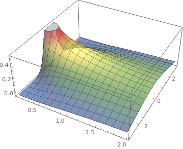
Plot3D[Erf[(x - 1/4)/Sqrt[4*t], (x + 1/4)/Sqrt[4*t]], {t, 0.1,
2}, {x, -3, 3}, ColorFunction -> "DarkRainbow",
PlotStyle -> Directive[Opacity[0.7], Red]]
Temperature distribution from hot spot.
Mathematica code
■
Example 4: Local solution of the heat equation
Example 4:
\begin{equation} \label{EqHeat.1}
\begin{split}
u_t &= u_{xx} , \qquad -\infty < x < \infty , \quad 0 < t < \delta , \\
u(x,0) &= f(x) , \qquad -\infty < x < \infty ,
\end{split}
\end{equation}
where
f (
x ) is a continuous function on ℝ.
The solution u (x, t ) of the initial value problem \eqref{EqHeat.1} gives the temperature distribution in an infinitely long homogeneous rod. If we set
\[
f(x) = e^{x^2} ,
\]
then the function
\[
u = u(x,t) = \left( 1 - 4t \right)^{-1/2} \exp\left\{ \frac{x^2}{1-4t} \right\}
\]
is the solution of the given IVP \eqref{EqHeat.1} for δ = 1/4, but it cannot be extended beyond the interval [0, 1/4].
■
The simplest initial-boundary value problem (IBVP) for an evolution PDE is the
problem on the half-line 0 < x < ∞, where the initial
condition u (x ,0) = f (x ) is supplemented with an
appropriate number (1 in our case) of boundary conditions at x = 0 and
u (x ,t ) decays as x ⟼ ∞ for all
t > 0. It is also assumed that the function u (x,t ) and its derivatives up to the second order are square integrable (we abbreviate it as u ∈ 𝔏²).. We consider three initial boundary value problems with boundary conditions of
Dirichlet, Neumann, and mixed types.
The Dirichlet problem for diffusion equation
The first problem to solve is the
following problem with Dirichlet boundary conditions:
\begin{align*}
&\mbox{Heat equation:} \qquad &u_t &= \alpha\,u_{xx} \qquad\mbox{for } x \in (0 ,\infty ) \mbox{ and } t > 0, \\
&\mbox{Initial condition:} \qquad &u(x,0) &= f(x) , \qquad x > 0, \\
&\mbox{Boundary condition:} \qquad &u(0,t) &= g(t) , \qquad t > 0 , \\
&\mbox{Regularity condition:} \qquad & \lim_{x \to \infty}\,|u(x,t) &= 0 , \quad\qquad u(x,t) \in 𝔏².
\end{align*}
The formulated Dirichlet problem can be solved with the aid of a sine Fourier transform. So we multiply both sides of the heat conduction equation by sin(
kx ) and integrate with respect to
x . This give
\[
\frac{{\text d}u^S}{{\text d}t} + \alpha\,k^2 u^S - k\,g(t) =0 , \qquad u^S (k,0) = f^S (k) ,
\]
where
\[
u^S (k,t) = \int_0^{\infty} u(x,t)\,\sin (kx)\,{\text d}x \qquad\mbox{and} \qquad f^S (k) = \int_0^{\infty} f(x)\,\sin (kx)\,{\text d}x .
\]
Its solution is
DSolve[{v'[t] + k^2 *v[t] - k*g[t] == 0, v[0] == f}, v[t], t]
{{v[t] ->
E^(k^2 t) (f +
Inactive[Integrate][-E^(-k^2 K[1]) k g[K[1]], {K[1], 0, t}])}}
\[
u^S (k,t) = f^S e^{-k^2 t} + k\, \int_0^t e^{-k^2 (t-\tau )} g(\tau )\,{\text d}\tau .
\]
Taking the inverse sine Fourier transform, we obtain the required solution formula:
Assuming[T > 0 && x > 0,
Integrate[k*Sin[k*x]*Exp[-k^2 *T], {k, 0, Infinity}]]*2/Pi
(E^(-(x^2/(4 T))) x)/(2 Sqrt[\[Pi]] T^(3/2))
\begin{align}
u(x,t) &=
\frac{2}{\pi} \int_0^{\infty} {\text d}k\,\sin (kx) \left[
e^{-k^2 t} \hat{f}^S (k) + k\int_0^t e^{-k^2 (t-\tau )} u(0,\tau )\,
{\text d}\tau \right] \notag
\\
&= \frac{x}{2\sqrt{\pi\alpha}} \, \int_0^t g(\tau )\left( t- \tau
\right)^{-3/2} e^{-x^2/4\alpha (t-\tau )}\,{\text d}\tau
+ \frac{1}{\pi\sqrt{\alpha\,t}} \int_0^{\infty} f(u) \left[
e^{-(x-u)^2 /(4\alpha t)} - e^{-(x+u)^2 /(4\alpha t)} \right] {\text d}u ,
\label{EqhFourier.2}
\end{align}
This formula provides an inadequate representation for the numerical evaluation of the solution because the spectral data is time-dependent (nonseparable).
This is a consequence of causality because the upper limit of the integral over the boundary data
u (0,
t ) is restricted to be
t rather than ∞.
Indeed, this follows from the limit
\[
\lim_{x\to 0}\,\frac{x}{2\sqrt{\pi\alpha}} \,s^{-3/2} e^{-x^2 /(4\alpha s)} =
\delta (s) , \qquad \mbox{Dirac delta function}.
\]
It is not straightforward to verify the boundary condition at
x =0: if we attempt to verify this condition by letting
x = 0 on the right hand side, we fail because sin 0 = 0 and
x is a multiplier. This implies that we cannot exchange the integration with the limit
x ↣0. Therefore, the convergence of the expression above to the delta function is understood in the weak sense, but not in the regular sense. This pathology (lack of uniform convergence at the boundary) is typical for any solution obtained via the Fourier transformations because its inverse is an example of an ill-posed problem.
Assuming[{x > 0 && a > 0 && s > 0},
Limit[x/2/Sqrt[a*Pi]*s^(-3/2)*Exp[-x^2/(4*a*s)], x -> 0]]
0
Assuming[{x > 0 && a > 0 && t > 0},
Integrate[
x/2/Sqrt[a*Pi]*s^(-3/2)*Exp[-x^2/(4*a*s)], {s, 0, Infinity}]]
1
Assuming[{x > 0 && a > 0 && t > 0},
Integrate[x/2/Sqrt[a*Pi]*s^(-3/2)*Exp[-x^2/(4*a*s)], {s, 0, t}]]
Erfc[x/(2 Sqrt[a t])]
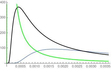
ff[x_, s_] = x/2/Sqrt[1*Pi]*s^(-3/2)*Exp[-x^2/(4*1*s)]
Three approximations of \( \frac{x}{2\sqrt{\alpha \pi}}\,
s^{-3/2} \,e^{-x^2 /(4\alpha s)} \)
Three approximations of \( \frac{x}{2\sqrt{\alpha \pi}}\,
s^{-3/2} \,e^{-x^2 /(4\alpha s)} \)
Mathematica code
The integral containing the boundary data g (t ) can be
transformed by substitution
\[
\tau = t - \frac{x^2}{4\alpha\,\eta^2} \qquad \Longrightarrow \qquad
{\text d}\tau = \frac{4\sqrt{\alpha}}{x} \left( t - \tau \right)^{3/2}
{\text d} \eta = \frac{x^2}{2\alpha} \,\eta^{-3} {\text d} \eta
\]
to
\[
\theta (x,t) = \frac{x}{2\sqrt{\pi\alpha}} \, \int_0^t g(\tau )\left( t- \tau
\right)^{-3/2} e^{-x^2/4\alpha (t-\tau )}\,{\text d}\tau =
\frac{2}{\sqrt{\pi}} \,\int_{v(x,t)}^{\infty} g \left( t -
\frac{x^2}{4\alpha\,\eta^2} \right) e^{-\eta^2} \,{\text d}\eta ,
\]
where
\( \displaystyle v(x,t) = \frac{x}{2\sqrt{\alpha\,t}} .
\)
From the latter, it follows that
\( \displaystyle \lim_{x\to 0} \, \theta (x,t) = g(t) \) because
2/Sqrt[Pi]*Integrate[ Exp[-t^2], {t, 0, Infinity}]
1
Proof:
We apply the sine Fourier transform to the given heat equation.
This yields
\[
\frac{{\text d}}{{\text d}t} \,\int_0^{\infty} u(x,t)\,\sin (kx)\,{\text d}x
= \alpha \int_0^{\infty} \frac{\partial^2 u(x,t)}{\partial x^2}\,\sin (kx)\,{\text d}x .
\]
Integrating by parts twice, we get
\[
ℱ_s \left[ \frac{{\text d}^2 f}{{\text d} x^2} \right] (k) =
\int_0^{\infty} \frac{\partial^2 u(x,t)}{\partial x^2}\,\sin (kx)\,{\text d}x =
\left. \frac{\partial u(x,t)}{\partial x}\,\sin (kx) \right\vert_{x=0}^{x=\infty} - \left. u(x,t) \,k\,\cos (kx) \right\vert_{x=0}^{x=\infty} - k^2
\int_0^{\infty} u(x,t)\,\sin (kx)\,{\text d}x .
\]
Assuming that the solution to the given initial boundary value problem tends to zero at infinity, we derive
\[
\int_0^{\infty} \frac{\partial^2 u(x,t)}{\partial x^2}\,\sin (kx)\,{\text d}x =
k\,u(0,t) - k^2 \int_0^{\infty} u(x,t)\,\sin (kx)\,{\text d}x .
\]
If we denote by
u S = ℱ
s [
u ] the sine Fourier transform of the (yet) unknown function
u (
x,t ) with respect to the variable
x , then
\[
\begin{split}
\frac{{\text d}}{{\text d}t}\, u^S + \alpha\,k^2 u^S &= \alpha\,k\,g(t) , \qquad t > 0,
\\
u^S (0) &= f^S (k) .
\end{split}
\]
Application of the Laplace transform yields
\[
\lambda \,U(k,\lambda ) + \alpha \,k^2 U(k,\lambda ) =
\alpha\,k\,g^L (\lambda ) + f^S (k) ,
\]
where
\[
U(k,\lambda ) = {\cal L} ℱ_s \left[ u(x,t) \right] = \int_0^{\infty}
u^S (k,t)\, e^{-\lambda\,t}\,{\text d}t \qquad\mbox{and} \qquad
g^L (\lambda ) = {\cal L} \left[ g(t) \right] = \int_0^{\infty}
g (t)\, e^{-\lambda\,t}\,{\text d}t
\]
are Laplace transforms of the functions
u S and
g ,
respectively. Solving the algebraic equation above for
U ,
we obtain
\[
U(k,\lambda ) = \frac{\alpha\,k}{\lambda + \alpha \,k^2}\,g^L (\lambda ) +
\frac{1}{\lambda + \alpha \,k^2}\,f^S (k) .
\]
Its inverse Laplace transform is
\[
u^S (k,t) = {\cal L}^{-1} \left[ U(k,\lambda ) \right] = \alpha\,k\,
e^{-\alpha\,k^2 t} * g(t) + f^S (k)\,e^{-\alpha\,k^2 t} =
\alpha\,k\,\int_0^t g(t-\tau )\,e^{-\alpha\,k^2 (t-\tau )} \,{\text d}\tau .
\]
Next, we apply the inverse sine Fourier transform to obtain
\[
\begin{split}
\frac{2}{\pi} \,\int_0^{\infty} \alpha\,k\,
e^{-\alpha\,k^2 t}\,\sin (kx)\, {\text d}k &= \frac{x}{2\,\sqrt{\pi\alpha}} \,
t^{-3/2} \,e^{-x^2 /(4\alpha\,t)} ,
\\
\frac{2}{\pi} \,\int_0^{\infty} e^{-\alpha\,k^2 t}\,\sin (kx)\, {\text d}k &=
\frac{2}{\pi\sqrt{\alpha t}} \, e^{- v^2 (x,t)} \int_0^{v(x,t)} e^{t^2} \,
{\text d}t ,
\end{split}
\]
where
\( \displaystyle v(x,t) = \frac{x}{2\sqrt{\alpha\,t}} .
\)
We check the answers with
Mathematica
Assuming[{t > 0 && aa > 0 && x > 0},
2/Pi*Integrate[k*Exp[-t*aa*k^2]*Sin[k*x], {k, 0, Infinity}]]
(E^(-(x^2/(4 aa t))) x (aa &))/(2 Sqrt[\[Pi]] (aa t)^(3/2))
Assuming[{t > 0 && aa > > && x > 0},
2/Pi*Integrate[Exp[-t*aa*k^2]*Sin[k*x], {k, 0, Infinity}]]
(2 DawsonF[x/(2 Sqrt[aa t])])/(\[Pi] Sqrt[aa t])
Here
Dawson's
integral is
\[
\mbox{Dawson}(x) = e^{-x^2} \int_0^x e^{\eta^2}\,{\text d}\eta .
\]
▣
Example 5: Dirichlet boundary conditions
Example 5:
\[
\begin{split}
u_t &= \alpha\, u_{xx} , \qquad x \in (0 ,\infty ), \quad t > 0,
\\
u(x,0) &= f(x) = x\,e^{-cx} ,
\\
u(0,t) &= g(t) = \sin (\omega t) .
\end{split}
\]
Using the sine Fourier transform, we get
Integrate[r*Exp[-c*r]*Sin[k*r] , {r, 0, Infinity}]
ConditionalExpression[(2 c k)/(c^2 + k^2)^2, Re[c] > Im[k]]
■
Example 6: Constant temperature at the boundary
Example 6:
\[
\begin{split}
u_t &= \alpha\, u_{xx} , \qquad x \in (0 ,\infty ), \quad t > 0,
\\
u(x,0) &= 0, \qquad x \in (0 ,\infty ),
\\
u(0,t) &= T_0 >0.
\end{split}
\]
This initial boundary value problem (IBVP) is ill-posed because the initial condition does match the boundary one. Of course, this problem does not sound right from a real world perspective. However, we use it for illustration.
Substituting the given data into the general formula, we obtain
\[
u(x,t) = \frac{x}{2\sqrt{\pi\alpha}} \, \int_0^t g(\tau )\left( t- \tau
\right)^{-3/2} e^{-x^2/4\alpha (t-\tau )}\,{\text d}\tau = \frac{x\, T_0}{2\sqrt{\pi\alpha}} \, \int_0^t e^{-x^2/4\alpha (t-\tau )}\,{\text d}\tau .
\]
Using
Mathematica , we find the value of the integral to be
Assuming[{t >0 && aa > 0 && x > 0},
Integrate[Exp[-x^2/aa/s]*s^(3/2), {s, 0, t}]]
(Sqrt[aa] Sqrt[\[Pi]] Erfc[x/Sqrt[aa t]])/x
\[
u(x,t) = \frac{T_0}{2\sqrt{\pi\alpha}} \,\sqrt{4\alpha\pi}\,\mbox{erfc} \left( \frac{x}{2\sqrt{\alpha\,t}} \right) = T_0 \mbox{erfc} \left( \frac{x}{2\sqrt{\alpha\,t}} \right) = T_0 \,\frac{2}{\sqrt{\pi}} \,\int_{x/(2\sqrt{\alpha t})} e^{-u^2}\,{\text d}u .
\]
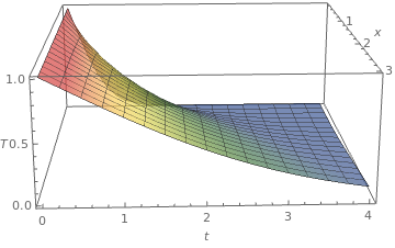
Plot3D[Erfc[(x)/Sqrt[4*t]], {t, 0.1, 3}, {x, 0, 4},
ColorFunction -> "DarkRainbow",
PlotStyle -> Directive[Opacity[0.7], Red], AxesLabel -> {x, t, T}]
Temperature distribution
Mathematica code
■
The Neumann problem for diffusion equation
The Neumann initial boundary value problem
\begin{align*}
&\mbox{Heat equation:} \qquad &u_t &= \alpha\,u_{xx} \qquad\mbox{for } x \in (0 ,\infty ) \mbox{ and } t > 0, \\
&\mbox{Initial condition:} \qquad &u(x,0) &= f(x) , \qquad x > 0, \\
&\mbox{Boundary condition:} \qquad &u_x (0,t) &= g(t) , \qquad t > 0 , \\
&\mbox{Regularity condition:} \qquad & \lim_{x \to \infty}\,|u(x,t) &= 0 , \quad\qquad u(x,t) \in 𝔏².
\end{align*}
can be solved with the aid of a cosine Fourier transform. So we multiply both sides of the heat conduction equation by cos(
xk ), integrate with respect to
x , then solve the resulting ordinary differential equation and obtain:
\begin{align*}
u(x,t) &=
\frac{2}{\pi} \int_0^{\infty} {\text d}k\,\cos (kx) \left[
\alpha \int_0^t e^{-k^2 (t-\tau )} u_x (0,\tau )\,
{\text d}\tau + e^{-k^2 t} \,\hat{f}^C (k) \right] .
\end{align*}
So integral evaluation yields
\begin{align}
u(x,t) &=
- \frac{\sqrt{\alpha}}{\sqrt{\pi}} \, \int_0^t g(\tau )\left( t- \tau
\right)^{-1/2} e^{-x^2/4\alpha (t-\tau )}\,{\text d}\tau
+ \frac{1}{2\sqrt{\pi\alpha\,t}} \int_0^{\infty} f(u) \left[
e^{-(x-u)^2 /(4\alpha t)} + e^{-(x+u)^2 /(4\alpha t)} \right] {\text d}u \notag
\\
&= -\frac{x}{\sqrt{\pi}} \,\int_{v(x,t)}^{\infty} g \left( t -
\frac{x^2}{4\alpha\,\eta^2} \right) e^{-\eta^2} \,\eta^{-2} {\text d}\eta +
\frac{1}{2\sqrt{\pi\alpha\,t}} \int_0^{\infty} f(u) \left[
e^{-(x-u)^2 /(4\alpha t)} + e^{-(x+u)^2 /(4\alpha t)} \right] {\text d}u ,
\label{EqhFourier.3}
\end{align}
where
\( \displaystyle \hat{f}^C (k) = ℱ_c \left[ f(x) \right) (k) = \int_0^{\infty} f(x)\,\cos (kx)\,{\text d}x \) is the cosine transform of the initial data
u (
x ,0) =
f (
x ) and
\( \displaystyle v(x,t) = \frac{x}{2\sqrt{\alpha\,t}} .
\)
Proof:
We apply the cosine Fourier transform to the given heat equation based on the
formula
\[
𝔉_c \left[ \frac{{\text d}^2 f}{{\text d} x^2} \right] (k) =
\int_0^{\infty} \frac{\partial^2 u(x,t)}{\partial x^2}\,\cos (kx)\,{\text d}x =
-u_x (0,t) - k^2 \int_0^{\infty} u(x,t)\,\cos (kx)\,{\text d}x .
\]
This yields the ordinary differential equation for the cosine Fourier transform
of the unknown function
\[
\begin{split}
\frac{{\text d}}{{\text d}t}\left( u^C \right)
+ \alpha\,k^2 u^C &= -\alpha\,g(t) , \qquad t > 0,
\\
u^C (0) &= f^C (k) ,
\end{split}
\]
where
\[
u^C (k,t) = \int_0^{\infty} u(x,t)\,\cos (kx)\,{\text d}x , \qquad
f^C (k) = ℱ_c \left[ f(x) \right] (k) = \int_0^{\infty} f(x)\,\cos (kx)\,{\text d}x .
\]
Application of the Laplace transform yields
\[
\lambda \,U(k,\lambda ) + \alpha \,k^2 U(k,\lambda ) =
-\alpha\,g^L (\lambda ) + f^S (k) ,
\]
where
\[
U(k,\lambda ) = {\cal L} ℱ_c \left[ u(x,t) \right] = \int_0^{\infty}
u^C (k,t)\, e^{-\lambda\,t}\,{\text d}t \qquad\mbox{and} \qquad
g^L (\lambda ) = {\cal L} \left[ g(t) \right] = \int_0^{\infty}
g (t)\, e^{-\lambda\,t}\,{\text d}t
\]
are Laplace transforms of the functions
u C and
g ,
respectively. Solving the algebraic equation above for
U ,
we obtain
\[
U(k,\lambda ) = \frac{-\alpha}{\lambda + \alpha \,k^2}\,g^L (\lambda ) +
\frac{1}{\lambda + \alpha \,k^2}\,f^C (k) .
\]
Its inverse Laplace transform is
\[
u^C (k,t) = {\cal L}^{-1} \left[ U(k,\lambda ) \right] = - \alpha\,
e^{-\alpha\,k^2 t} * g(t) + f^C (k)\,e^{-\alpha\,k^2 t} =
\alpha\,\int_0^t g(t-\tau )\,e^{-\alpha\,k^2 (t-\tau )} \,{\text d}\tau +
f^C (k)\,e^{-\alpha\,k^2 t} .
\]
Next, we apply the inverse cosine Fourier transform to obtain
\[
\begin{split}
\frac{2}{\pi} \,\int_0^{\infty} e^{-\alpha\,k^2 t}\,\cos (kx)\, {\text d}k &=
\frac{1}{\sqrt{\alpha\pi\,t}} \, e^{-x^2 /(4\alpha\,t)} .
\end{split}
\]
Assuming[{t > 0 && aa > 0 && x > 0},
2/Pi*Integrate[ aa *Exp[-t*aa*k^2]*Cos[k*x], {k, 0, Infinity}]]
(aa E^(-(x^2/(4 aa t))))/(Sqrt[\[Pi]] Sqrt[aa t])
Using the generalized convolution rule
\begin{align*}
\left( f \overset{0}{*} g \right) (x) &= \int_0^{\infty} f(y)
\left[ g(|x-y|) + g(x+y) \right] {\text d}y ,
\end{align*}
we arrive at the required formula.
■
Example 7: Neumann boundary conditions for heat equation
Example 7:
\[
\begin{split}
u_t &= \alpha\, u_{xx} , \qquad x \in (0 ,\infty ), \quad t > 0,
\\
u(x,0) &= f(x) = x\,e^{-cx} ,
\\
u_x (0,t) &= g(t) = \sin (\omega t) ,
\end{split}
\]
where
c and ω are positive constants.
Using the cosine Fourier transform, we get
Integrate[r*Exp[-c*r]*Cos[k*r] , {r, 0, Infinity}]
ConditionalExpression[((c - k) (c + k))/(c^2 + k^2)^2, Re[c] > Im[k]]
\[
\begin{split}
\frac{{\text d}}{{\text d}t}\, u^C + \alpha\,k^2 u^C &= -\alpha\,g(t) , \qquad
t > 0,
\\
u^C (0) &= f^C (k) = \frac{c^2 - k^2}{\left( c^2 + k^2 \right)^2} ,
\end{split}
\]
where
\[
u^C (k,t) = \int_0^{\infty} u(x,t)\,\cos (kx)\,{\text d}x , \qquad
f^C (k) = ℱ_c \left[ f(x) \right] (k) = \int_0^{\infty} x\,e^{-cx},\cos (kx)\,{\text d}x = \frac{c^2 - k^2}{\left( c^2 + k^2 \right)^2} .
\]
Next, we apply the Laplace transform to obtain the algebraic equation
\[
\lambda\, U(k,\lambda ) + \alpha\,k^2 U(k, \lambda ) =
-\alpha\, g^L (\lambda ) + f^C (k)
\]
for
\[
U(k, \lambda ) = {\cal L}ℱ_c \left[ u(x,t) \right] = \int_0^{\infty}
u^C (k,t)\, e^{-\lambda\,t}\,{\text d}t .
\]
LaplaceTransform[Sin[omega*t], t, s]
omega/(omega^2 + s^2)
Solving for
U , we obtain
\[
U(k, \lambda ) = - \frac{\alpha}{\lambda + \alpha\, k^2} \,g^L +
\frac{f^C (k)}{\lambda + \alpha\, k^2} =
- \frac{\alpha}{\lambda + \alpha\, k^2} \,\frac{\omega}{\lambda^2 + \omega^2}
+ \frac{f^C (k)}{\lambda + \alpha\, k^2} .
\]
Using the inverse Laplace transform, we get
\[
u^C (k,t) = -\frac{\alpha\omega}{\omega^2 + \alpha^2 k^4}\, e^{-\alpha k^2 t} -
\frac{\alpha}{\alpha^2 k^4 + \omega^2} \left[ \alpha\,k^2 \sin (\omega t) -
\omega\,\cos (\omega t) \right] + \frac{c^2 - k^2}{\left( c^2 + k^2 \right)^2}
\,e^{-\alpha k^2 t} .
\]
InverseLaplaceTransform[1/(s + aa)*omega/(s^2 + omega^2), s, t]
omega (E^(-aa t)/(
aa^2 + omega^2) + (-omega Cos[omega t] + aa Sin[omega t])/(
omega (aa^2 + omega^2)))
Finally, we apply the inverse cosine Fourier transform to obtain the
required solution:
\[
u(x,t) = ℱ_c^{-1} \left[ u^C (k, t) \right] = \frac{2}{\pi} \,
\int_0^{\infty} u^C (k, t) \,\cos (kx) \,{\text d}k .
\]
Substituting the explicit expressions and using formulas
\[
\frac{2}{\pi} \int_0^{\infty} {\text d}k\, \cos (kx)\,\frac{1}{\omega^2 + \alpha^2 k^4}\, e^{- \alpha k^2 t} = ??
\]
\[
u(x,t) = \left( ℱ_c \right)^{-1} \left[ u^C (k, t) \right] 𝔉_c^{-1}
\]
we obtain
■
The mixed boundary value problem for diffusion equation
Consider the diffusion equation on the half-line with a
mixed boundary
condition at
x = 0:
\begin{align*}
&\mbox{Heat equation:} \qquad &u_t &= \alpha\,u_{xx} \qquad\mbox{for } x \in (0 ,\infty ) \mbox{ and } t > 0, \\
&\mbox{Initial condition:} \qquad &u(x,0) &= f(x) , \qquad x > 0, \\
&\mbox{Boundary condition:} \qquad &a\,u(0,t) - b\,u_x (0,t) &= g(t) , \qquad t > 0 , \\
&\mbox{Regularity condition:} \qquad & \lim_{x \to \infty}\,|u(x,t) &= 0 , \quad\qquad u(x,t) \in 𝔏².
\end{align*}
where
\( u_t = \partial u/\partial t , \quad u_x =
\partial u/\partial x , \quad u_{xx} = \partial^2 u/\partial x^2 \)
are partial derivatives of the unknown function
u (
x, t ).
Here
f (
x ) and
g (
t ) are prescribed functions
decaying sufficiently fast for large
x and
t , respectively.
The conventional method for solving this
problem is to use the generalized Fourier transforms. We have
\[
\hat{u} (k,t) = \int_0^{\infty} \left[ \cos (kx) + \frac{a}{bk}\,\sin (kx)
\right] u(x,t)\,{\text d}x .
\]
Substitution into the diffusion equation and integration by parts yields an
equation for
\( \hat{u} : \)
\[
\frac{{\text d} \hat{u} (k,t)}{{\text d} t} + \alpha\,k^2 \hat{u} (k,t) = \alpha \left[ - u_x (0,t) +
\frac{a}{b}\,u(0,t) \right] = \alpha\,g(t)/b .
\]
We supply the initial condition for
\( \hat{u} \)
by applying the generalized Fourier transform to the initial condition
\( u(x,0) = f(x) . \) This leads to
\[
\hat{u} (k,0) = \hat{f} (k) , \qquad \mbox{where} \quad \hat{f} (k) =
\int_0^{\infty} \left[ \cos (kx) + \frac{a}{bk}\,\sin (kx)
\right] f(x)\,{\text d}x .
\]
With
Mathematica , we find the solution to the initial value problem
DSolve[{v'[t] + k^2 *v[t] - g[t] == 0, v[0] == f}, v[t], t]
{{v[t] ->
E^(-k^2 t) (f +
Inactive[Integrate][E^(k^2 K[1]) g[K[1]], {K[1], 0, t}])}}
\[
\hat{u} (k,t) = \hat{f}\,e^{-\alpha k^2 t} + \alpha \int_0^t e^{-\alpha k^2 (t-\tau )} \left[ - u_x (0,\tau ) +
\frac{a}{b}\,u(0,\tau ) \right] {\text d}\tau .
\]
Nevertheless, we solve the preceding initial value problem with the aid of the Laplace transformation
in
t :
\[
\left( \lambda + \alpha\,k^2 \right) \hat{u}^L (k,\lambda ) = \alpha\,g^L (\lambda )/b +
\hat{f} (k) ,
\]
where
\[
\hat{u}^L (k,\lambda ) = {\cal L} \left[ \hat{u} (k,t) \right] (\lambda ) =
\int_0^{\infty} \hat{u} (k,t) \, e^{-\lambda t} \,{\text d} t , \qquad
g^L (\lambda ) = {\cal L} \left[ g (t) \right] (\lambda ) =
\int_0^{\infty} g (t) \, e^{-\lambda t} \,{\text d} t
\]
are Laplace transforms of functions
\( \hat{u} \)
and
g , respectively. Application of the inverse Laplace transform yields
\[
\hat{u} (k,t ) = {\cal L}^{-1} \left[ \hat{u}^L (k,\lambda ) \right] =
{\cal L}^{-1} \left[ \frac{\alpha\,g^L (\lambda )/b + \hat{f} (k)}{\lambda + \alpha\,k^2}
\right] = \frac{\alpha}{b}\, g* e^{-\alpha k^2 t} + \hat{f} (k)\, e^{-\alpha k^2 t} ,
\]
where the asterisk denotes the convolution operation:
\[ \
g* e^{-k^2 t} = \int_0^{t} g(\tau )\,e^{-\alpha\,k^2 (t-\tau )} \,{\text d} \tau .
\]
Now we apply the inverse Fourier transform to obtain
\begin{align*}
u(x,t) &= \frac{2}{\pi} \int_0^{\infty} \hat{u} (k,t)\,\frac{k^2}{a^2 /b^2 + k^2}
\left[ \cos (kx) + \frac{a}{kb}\,\sin (kx)
\right] {\text d}k
\\
&= \frac{2\alpha}{b\,\pi}\,
\int_0^{t} g(\tau )\,{\text d}\tau\, \int_0^{\infty}
e^{-\alpha k^2 (t-\tau )}\,\frac{k^2}{a^2 /b^2 + k^2}
\left[ \cos (kx) + \frac{a}{kb}\,\sin (kx)
\right] {\text d}k + \frac{2}{\pi}\, \int_0^{\infty} \hat{f} (k)\, e^{-\alpha k^2 t}
\, \frac{k^2}{a^2 /b^2 + k^2}
\left[ \cos (kx) + \frac{a}{kb}\,\sin (kx)
\right] {\text d}k .
\end{align*}
Unfortunately,
Mathematica does not know how to evaluate these integrals. So we simplify them a little bit
\begin{align*}
u(x,t) &= \frac{2\alpha}{b\,\pi}\,
\int_0^{t} g(\tau )\,{\text d}\tau\, \int_0^{\infty} e^{-\alpha k^2 (t-\tau )}\,\frac{k^2}{a^2 /b^2 + k^2} \, \cos (kx) \, {\text d}k +
\frac{2a\,\alpha}{b\,\pi}\,
\int_0^{t} g(\tau )\,{\text d}\tau\, \int_0^{\infty} e^{-\alpha k^2 (t-\tau )}\,\frac{k}{a^2 /b^2 + k^2} \, \sin (kx) \, {\text d}k
\\
&\quad + \frac{2}{\pi}\, \int_0^{\infty} f (u)\,{\text d}u \int_0^{\infty} e^{-\alpha k^2 t}
\, \frac{k^2}{a^2 /b^2 + k^2} \left[ \cos (ku) + \frac{a}{kb}\,\sin (ku)
\right] \left[ \cos (kx) + \frac{a}{kb}\,\sin (kx)
\right] {\text d}k .
\tag{Integral.1}
\end{align*}
The right-hand side is expressed through two intregrals:
\begin{align*}
C(a,T,x) &= \int_0^{\infty} e^{-T\,k^2} \,\frac{k^2 \cos (kx)}{a^2 + k^2} \,{\text d}k ,
\tag{Integral.2}
\\
S(a,T,x) &= \int_0^{\infty} e^{-T\,k^2} \,\frac{k\, \sin (kx)}{a^2 + k^2} \,{\text d}k .
\tag{Integral.3}
\end{align*}
Then
\begin{align}
u(x,t) &=
\frac{2\alpha}{b\,\pi}\,
\int_0^{t} g(\tau )\,{\text d}\tau \left[ C \left( \frac{a}{b} , x, t - \tau \right) + \frac{a}{b} \,S \left( \frac{a}{b} , x, t - \tau \right) \right]
\notag
\\
&\quad + \frac{1}{\pi} \int_0^{\infty} f (u)\,{\text d}u \left[ C \left( \frac{a}{b} , u-x, t \right) + \frac{a^2}{b^2} \, A \left( \frac{a}{b} , u-x, t \right) + \frac{a^2}{b^2} \, A \left( \frac{a}{b} , u+x, t \right) + \frac{2a}{b}\,S \left( \frac{a}{b} , u+x, t \right) \right] ,
\label{EqhFourier.4}
\end{align}
because
TrigReduce[(Cos[X] + A*Sin[X])*(Cos[Y] + A*Sin[Y])]
1/2 (Cos[X - Y] + A^2 Cos[X - Y] + Cos[X + Y] - A^2 Cos[X + Y] +
2 A Sin[X + Y])
Evaluation of Integral C (𝑎,T,x )
By adding and subtracting 𝑎² in the numerator, we obtain
\[
C(a,T,x) = \int_0^{\infty} e^{-T\,k^2} \,\frac{\left( k^2 + a^2 - a^2 \right) \cos (kx)}{a^2 + k^2} \,{\text d}k = \int_0^{\infty} e^{-T\,k^2} \,\cos (kx)\,{\text d}k - a^2 \int_0^{\infty} e^{-T\,k^2} \,\frac{\cos (kx)}{a^2 + k^2} \,{\text d}k .
\]
The first integral is evaluated with the aid of
Mathematica :
Assuming[ a > 0 && x > 0 && T > 0,
Integrate[Exp[-T*k^2]*Cos[k*x], {k, 0, Infinity}]]
(E^(-(x^2/(4 T))) Sqrt[\[Pi]])/(2 Sqrt[T])
\[
\int_0^{\infty} e^{-T\,k^2} \,\cos (kx)\,{\text d}k = \frac{\sqrt{\pi}}{2\sqrt{T}} \, e^{-x^2 /(4T)} .
\]
In order to evaluate the latter, we introduce the auxiliary integral
\[
A(a,T,x) = \int_0^{\infty} e^{-T\,k^2} \,\frac{\cos (kx)}{a^2 + k^2} \,{\text d}k .
\]
Then the required integral will be explicitly expressed as
\[
C(a,T,x) = \frac{\sqrt{\pi}}{2\sqrt{T}} \, e^{-x^2 /(4T)} - a^2 A(a,T,x) .
\]
Multiplying
A (𝑎,
T,x ) by
\( \displaystyle e^{-a^2 T} \) and diferentiating with respect to
T , we obtain
\[
\frac{\text d}{{\text d}T} e^{-a^2 T} \,A(a,T,x) = \frac{\text d}{{\text d}T} \int_0^{\infty} e^{-T\left( k^2 + a^2 \right)} \,\frac{\cos (kx)}{a^2 + k^2} \,{\text d}k = - e^{-a^2 T} \,\int_0^{\infty} e^{-T\,k^2} \,\cos (kx) \,{\text d}k = - e^{-a^2 T} \, \frac{\sqrt{\pi}}{2\sqrt{T}} \, e^{-x^2 /(4T)} .
\]
This is a simple differential equation, which we solve by
Integration
Assuming[ a > 0 && x > 0 && t > 0,
Integrate[(E^(-(x^2/(4 T))) Sqrt[\[Pi]])/(2 Sqrt[T])*Exp[-a^2 *T],{T,0,t}]]
-(E^(-a x) \[Pi] (-2 + Erfc[-((-2 a t + x)/(2 Sqrt[t]))] +
E^(2 a x) Erfc[(2 a t + x)/(2 Sqrt[t])]))/(4 a)
\[
e^{-a^2 T} \,A(a,T,x) = - \int_0^{T} e^{-a^2 T} \, \frac{\sqrt{\pi}}{2\sqrt{T}} \, e^{-x^2 /(4T)} \, {\text d} T =
-\frac{\pi}{2a}\, e^{-ax} + \frac{\pi}{4a}\,e^{-ax} \,\mbox{Erfc} \left( \frac{2aT-x}{2\sqrt{T}} \right) + \frac{\pi}{4a}\,e^{ax} \,\mbox{Erfc} \left( \frac{2aT+x}{2\sqrt{T}} \right) .
\]
Since
\[
A(a,0,x) = \int_0^{\infty} \frac{\cos (kx)}{a^2 + k^2} \,{\text d}k = \frac{\pi}{2a}\,e^{-ax} ,
\]
Assuming[a > 0 && x > 0 && T > 0,
Integrate[Cos[k*x]/(a^2 + k^2), {k, 0, Infinity}]]
(E^(-a x) \[Pi])/(2 a)
we get
\[
A(a,T,x) =
-\frac{\pi}{2a}\, e^{-ax + a^2 T} + \frac{\pi}{4a}\,e^{-ax + a^2 T} \,\mbox{Erfc} \left( \frac{2aT-x}{2\sqrt{T}} \right) + \frac{\pi}{4a}\,e^{ax+ a^2 T} \,\mbox{Erfc} \left( \frac{2aT+x}{2\sqrt{T}} \right) .
\]
▣
\[
C(a,T,x) = \frac{\sqrt{\pi}}{2\sqrt{T}} \, e^{-x^2 /(4T)} - \frac{\pi a}{4}\,e^{a^2 T} \left\{ e^{-ax}\, \mbox{Erfc} \left( \frac{2aT-x}{2\sqrt{T}} \right) + e^{ax}\, \mbox{Erfc} \left( \frac{2aT+x}{2\sqrt{T}} \right) \right\} + \frac{\pi a}{2}\,e^{a^2 T -ax} .
\tag{Integral.2a}
\]
Evaluation of Integral S (𝑎,T,x )
We immediately find
\begin{align*}
S(a,T,x) &= \int_0^{\infty} e^{-T\,k^2} \,\frac{k\, \sin (kx)}{a^2 + k^2} \,{\text d}k = - \frac{\text d}{{\text d}x} \int_0^{\infty} e^{-T\,k^2} \,\frac{\cos (kx)}{a^2 + k^2} \,{\text d}k
= - \frac{\text d}{{\text d}x} \,A(a,T,x)
\\
&= \frac{\pi}{4}\,e^{a^2 T -a x} \, \mbox{Erfc} \left( \frac{2aT-x}{2\sqrt{T}} \right) + \frac{\pi}{4}\,e^{a^2 T -a x} \, \mbox{Erfc} \left( \frac{2aT+x}{2\sqrt{T}} \right) - \frac{\pi}{2}\,e^{a^2 T -ax}
\\
&\quad + \frac{\pi}{4a}\,e^{a^2 T - ax} \, \frac{\text d}{{\text d}x} \left\{ \mbox{Erf} \left( \frac{2aT-x}{2\sqrt{T}} \right) + \mbox{Erf} \left( \frac{2aT+x}{2\sqrt{T}} \right) \right\} .
\end{align*}
Since
D[Erfc[x], x]
-((2 E^-x^2)/Sqrt[\[Pi]])
\[
\frac{\text d}{{\text d}x} \,\mbox{Erfc} \left( x \right) = - \frac{2}{\sqrt{\pi}} \, e^{-x^2} ,
\]
then
\[
\frac{\text d}{{\text d}x} \,\mbox{Erfc} \left( \frac{2aT-x}{2\sqrt{T}} \right) = \frac{1}{\sqrt{\pi\, T}} \, e^{- \left( 2aT -x \right)^2 /(4T)} , \qquad \frac{\text d}{{\text d}x} \,\mbox{Erfc} \left( \frac{2aT-x}{2\sqrt{T}} \right) = -\frac{1}{\sqrt{\pi\, T}} \, e^{- \left( 2aT +x \right)^2 /(4T)} .
\]
D[Erfc[(2*a*T -x)/2/Sqrt[T]], x]
E^(-((2 a T - x)^2/(4 T)))/(Sqrt[\[Pi]] Sqrt[T])
D[Erfc[(2*a*T +x)/2/Sqrt[T]], x]
-(E^(-((2 a T + x)^2/(4 T)))/(Sqrt[\[Pi]] Sqrt[T]))
Therefore,
\begin{align*}
S(a,T,x) &= \frac{\pi}{4}\,e^{a^2 T -a x} \, \mbox{Erfc} \left( \frac{2aT-x}{2\sqrt{T}} \right) + \frac{\pi}{4}\,e^{a^2 T -a x} \, \mbox{Erfc} \left( \frac{2aT+x}{2\sqrt{T}} \right) - \frac{\pi}{2}\,e^{a^2 T -ax}
\\
&\quad + \frac{\sqrt{\pi}}{4a\sqrt{T}} \,,e^{a^2 T -a x} \left[ e^{- \left( 2aT -x \right)^2 /(4T)} - e^{- \left( 2aT +x \right)^2 /(4T)} \right] .
\end{align*}
▣
\begin{align*}
S(a,T,x) &= \frac{\pi}{4}\,e^{a^2 T -a x} \, \mbox{Erfc} \left( \frac{2aT-x}{2\sqrt{T}} \right) + \frac{\pi}{4}\,e^{a^2 T -a x} \, \mbox{Erfc} \left( \frac{2aT+x}{2\sqrt{T}} \right) - \frac{\pi}{2}\,e^{a^2 T -ax}
\\
&\quad + \frac{\sqrt{\pi}}{4a\sqrt{T}} \,,e^{a^2 T -a x} \left[ e^{- \left( 2aT -x \right)^2 /(4T)} - e^{- \left( 2aT +x \right)^2 /(4T)} \right] .
\tag{Integral.3a}
\end{align*}
Example 8: Mixed boundary conditions for heat equation
Example 8:
\[
\begin{split}
u_t = \alpha\, u_{xx} , \qquad x,t \in (0,\infty ),
\\
a\,u(0,t) - b\,u_x (0,t) = g(t) = \sin (\omega t) , \\
u(x,0) = f(x) = x\,e^{-cx} ,
\end{split}
\]
where
c and ω are positive constants.
■
References
Barton, G. Elements of Green's Functions and Propagation: Potentials, Diffusion, and Waves , [Reprint] (Oxford Science Publications)
Bressloff, P.C., A new Green's function method for solving linear PDEs in two variables , Journal of Mathematical Analysis and Applications , 1997, Vol. 210, Issue 1, pp. 390--415.
F. Calogero and S. De Lillo, The Burgers equation on the semiline with general boundary conditions at the origin, Journal of Mathematical Physics, Vol. 32, Issue 1, pp. 99‑105 (1991).
Doniach, S. and Sondheimer, E.,
Green's Functions for Solid State Physicists , Reprint Edition, 1998,
Imperial College Pr;
Jentschura. U.D., Advanced Classical Electrodynamics: Green Functions, Regularizations, Multipole Decompositions , 2017, World Scientific Pub Co Inc.
Roach, G.F., Green's Functions , 2nd edition, 1982, Cambridge University Press
Thao, N.X., Kakichev, V.A., Tuan, V.K., On the generalized convolution for Fourier cosine and sine transforms, East-West Journal of Mathematics , 1998, Vol. 1, No. 1, pp. 85--90.
Return to Mathematica page main page (APMA0340) Part 1 Matrix Algebra Part 2 Linear Systems of Ordinary Differential Equations Part 3 Non-linear Systems of Ordinary Differential Equations Part 4 Numerical Methods Part 5 Fourier Series Part 6 Partial Differential EquationsPart 7 Special Functions