Return to computing page for the first course APMA0330
Return to computing page for the second course APMA0340
Return to Mathematica tutorial for the first course APMA0330
Return to Mathematica tutorial for the second course APMA0340
Return to the main page for the first course APMA0330
Return to the main page for the second course APMA0340
Return to Part V of the course APMA0340
Introduction to Linear Algebra with Mathematica

Preface


Pafnuty Chebyshev

Laguerre's polynomials,

\begin{equation} \label{EqLaguerre.1} L_n (x) = \sum_{k=0}^n (-1)^k \binom{n}{k} \frac{x^k}{k!} , \qquad n=0,1,2,\ldots , \end{equation}
are eigenfunctions corresponding to eigenvalues λ = n∈ ℕ = {0, 1, 2, …}, of the singular Sturm--Liouville problem on the half-line (0, ∞):
\begin{equation} \label{EqLaguerre.2} x\,y'' + \left( 1 -x \right) y' + \lambda\,y = 0, \qquad y(0) < \infty , \end{equation}
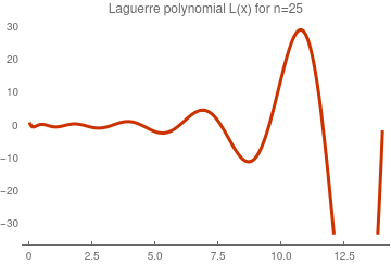
where \( \displaystyle \binom{n}{k} = \frac{n^{\underline{k}}}{k!} \) are binomial coefficients and \( \displaystyle n^{\underline{k}} = n\cdot (n-1) \cdot (n-2) \cdots (n-k+1) \) is n-th falling factorial. Since the Chebyshev--Laguerre equation \eqref{EqLaguerre.2} has a regular singular point at the origin, it has a regular (polynomial) solution only when λ is a nonnegative integer. The polynomial solutions for λ = n ∈ ℕ were invented by the Russian mathematician Pafnuty Chebyshev (1821--1894) in 1859. These solutions were known in nineteen century as Chebyshev--Laguerre polynomials.

Actually, there is no evidence that Edmond Laguerre contributed to differential equation \eqref{EqLaguerre.2} and analyzed or obtained its solutions that bare his name. In 1879, Edmond Nicolas Laguerre (1834--1886) studied exponential integral (now abbreviated as \( {\mbox Ei}(x) = \int_x^{+\infty} \frac{e^t}{t}\,{\text d}t \) ) and utilized the corresponding differential equation

\[ x\,u'' + \left( 1 +x \right) u' - n\,u = 0, \qquad n\in \mathbb{N} = \left\{ 0,1,2,\ldots \right\} , \]
but not the Chebyshev--Laguerre equation \eqref{EqLaguerre.2}. See a historical note by M.E. Hassani. However, the differential equation considered by Laguaerre in 1879 has a solution that is similar to \eqref{EqLaguerre.1}:
\[ u(x) = \sum_{k=0}^n \binom{n}{k} \frac{x^k}{k!} , \qquad n=0,1,2,\ldots . \]

In 1880, a Russian mathematician Nikolay Yakovlevich Sonin (1849--1915) invented a generalization of the Chebyshev--Laguerre equation

\begin{equation} \label{EqLaguerre.3} x\,y'' + \left( \alpha + 1 -x \right) y' + \lambda\,y = 0, \qquad y(0) < \infty . \end{equation}
He analyzed its solutions for arbitrary real α > −1 and showed that when λ = n, an integer (eigenvalue), it has a polynomial solution that now is known as a generalized Laguerre polynomial or Sonin polynomial. For eigenvalues λ = n ∈ ℕ, these polynomials are denoted by \( L_n^{(\alpha )} (x) \) or \( L_n^{\alpha} (x) \) or L(α, x).


Laguerre Equation


Edmond Laguerre

The Laguerre polynomials, Ln(x), are solutions of the Chebyshev--Laguerre differential equation

\[ x\,y'' + \left( 1-x \right) y' +n\,y =0, \quad\mbox{or} \quad \frac{{\text d}}{{\text d} x} \left( x\,e^{-x} \,y' \right) + n\,e^{-x}\,y =0 , \qquad x\in (0,\infty ). \]
This second order linear differential equation has a regular singular point at the origin (where the leading coefficient vanishes) and irregular singular point at infinity. Every Laguerre polynomial Ln(x) is a polynomial of degree n, so it is bounded at the origin x = 0. The general solution of Eq.\eqref{EqLaguerre.2} is a linear combination of two functions
\[ y (x) = C_1 L_n (x) + C_2 Q_n (x) , \]
where Qn(x) is another solution that is unbounded at the origin.

The Laguerre polynomial may be defined by the Rodrigues formula (the French banker Olinde Rodrigues (1795--1851) defined it in 1816)

\[ L_n (x) = \frac{e^x}{n!} \, \frac{{\text d}^n}{{\text d} x^n} \left( x^n e^{-x} \right) = \frac{1}{n!} \left( \frac{{\text d}}{{\text d} x} - 1 \right) x^n , \qquad n=0,1,2,\ldots . \]
These polynomials can be obtained from the ordinary generating function
\[ \left( 1 - x \right)^{-1} e^{xt/(t-1)} = \sum_{n\ge 0} L_n (x)\,t^n , \qquad |t| < 1. \]

Although Mathematica has a dedicated command LaguerreL for evaluation Laguerre polynomials, we find first ten these polynomials from its ordinary generating function:

Series[Exp[-x*t/(1 - t)]/(1 - t), {t, 0, 10}]
SeriesCoefficient[Exp[-x*t/(1 - t)]/(1 - t), {t, 0, 3}]
       n     Laguerre polynomial
    n = 0         L0(x) = 1
    n = 1         L1(x) = 1 − x
    n = 2         \( \displaystyle L_2 (x) = \frac{1}{2} \left( x^2 - 4x + 2 \right) \)
    n = 3         \( \displaystyle L_3 (x) = \frac{1}{6} \left( - x^3 + 9 x^2 -18x + 6 \right) \)
    n = 4         \( \displaystyle L_4 (x) = \frac{1}{4!} \left( x^4 -16 x^3 + 72\,x^2 -96\,x + 24 \right) \)
    n = 5         \( \displaystyle L_5 (x) = \frac{1}{5!} \left( - x^5 +25\, x^4 -200\,x^3 + 600\, x^2 -600\,x + 120 \right) \)
    n = 6         \( \displaystyle L_6 (x) = \frac{1}{6!} \left( x^6 - 36\,x^5 + 450\, x^4 -2400\,x^3 + 5400\, x^2 -4320\,x + 720 \right) \)
    n = 7         \( \displaystyle L_7 (x) = \frac{1}{7!} \left( - x^7 +49\,x^6 - 882\, x^5 + 7350\,x^4 -29400\, x^3 + 52920\,x^2- 35280\,x +5040 \right) \)
    n = 8         \( \displaystyle L_8 (x) = \frac{1}{8!} \left( x^8 - 64\,x^7 +1568\, x^6 - 18816\,x^5 + 117600\, x^4 + 376320\,x^3 + 564480\, x^2 -322560\,x + 40320 \right) \)
    n = 9         \( \displaystyle L_9 (x) = \frac{1}{9!} \left( - x^9 + 81\,x^8 - 2592 x^7 + 42366\,x^6 - 381024\, x^5 + 1905120\,x^4 - 5080320\,x^3 x^3 + 6531840\,x^2 - 3265920\. x + 362880 \right) \)
    n = 10         \( \displaystyle L_{10} (x) = \frac{1}{10!} \left( x^{10} - 100\,x^9 +4050\,x^8 x^8 -86400\,x^7 + 1058400\, x^6 - 7620480\,x^5 + 31752000\, x^4 - 72576000\,x^3 + 81648000\, x^2 - 36288000\,x + 3628800 \right) \)

Example 1: Using Mathematica, we plot some Laguerre polynomials

Plot[LaguerreL[5, x], {x, 0, 7}, PlotTheme -> "Web", PlotLabel -> "Laguerre polynomial L(x) for n=5"]
Plot[LaguerreL[12, x], {x, 0, 15}, PlotTheme -> "Web", PlotLabel -> "Laguerre polynomial L(x) for n=12"]
Plot[LaguerreL[25, x], {x, 0, 14}, PlotTheme -> "Web", PlotLabel -> "Laguerre polynomial L(x) for n=25"]
       
       
Laguerre polynomial L5(x)         Laguerre polynomial L12(x)         Laguerre polynomial L25(x)


Recurrences


One can also define the Laguerre polynomials recursively,
\[ L_{n+1} (x) = \frac{1}{n+1} \left[ \left( 2n+1-x \right) L_n (x) -n\,L_{n-1} \right] , \quad L_0 (x) =1, \quad L_1 (x) = 1-x, \quad n=1,2,3,\ldots . \tag{R.1} \]
((2*7 + 1 - x)*LaguerreL[7, x] - 7*LaguerreL[6, x])/(7 + 1)
Simplify[% - LaguerreL[8, x]]
For derivatives, we have
\[ L'_{n+1} (x) - L'_n (x) + L_{n} (x) = 0 , \quad L_0 (x) =1, \quad L_1 (x) = 1-x, \quad n=0,1,2,3,\ldots . \tag{R.2} \]
Simplify[D[LaguerreL[9, x], x] - D[LaguerreL[8, x], x] + LaguerreL[8, x]]
\[ x\,L'_{n} (x) - n\, L_n (x) +n\,L_{n-1} (x) = 0 , \quad L_0 (x) =1, \quad L_1 (x) = 1-x, \quad n=2,3,\ldots . \tag{R.3} \]
Simplify[x*D[LaguerreL[9, x], x] - 9*LaguerreL[9, x] + 9*LaguerreL[8, x]]
\[ \frac{\text d}{{\text d}x}\, L_n (x) = \left( \frac{\text d}{{\text d}x} -1 \right) L_{n-1} (x) , \qquad n=1,2,\ldots . \]

Arbitrary function for which the integral

\[ \| f \|^2 = \int_0^{\infty} e^{-x} |f(x)|^2 {\text d} x < \infty \]
converges, can be expanded into Laguerre series:
\begin{equation} \label{EqLaguerre.4} f(x) = \sum_{i\ge 0} f_i L_i (x) , \qquad f_i = \int_0^{\infty} L_i (x) \,e^{-x} f(x) \, {\text d} x , \qquad i=0,1,2,\ldots , \end{equation}
which converges in 𝔏p(ℝ+, e−x) for \( p \in \left( \frac{4}{3} , 4 \right) . \) Such expansion is based on the orthogonal property of Laguerre polynomials:
\[ \int_0^{\infty} L_n (x) \,L_m (x) \, e^{-x} \, {\text d} x = \delta_{n,m} \equiv \begin{cases} 1 , & \quad \mbox{if $n=m$}, \\ 0 , & \quad \mbox{if $n\ne m$}. \end{cases} \]

Since a set of Laguaerre polynomials { Ln(x) }n∈ℕ form a complete orthogonal system in the Hilbert space 𝔏²(ℝ, e−x), the coefficients fi of expansion \eqref{EqLaguerre.4} satisfy Parseval's identity (it can be extended for complex-values functions):

\[ \| f \|^2 = \int_0^{\infty} \left\vert f (x)\right\vert^2 e^{-x} {\text d} x = \sum_{n\ge 0} f^2_i . \]


Some Useful Formulas


The Laguerre polynomials are closely related to the incomplete gamma functions; there are two of them: the upper incomplete gamma function
\[ \Gamma (\nu , x) = \int_x^{\infty} t^{\nu -1} e^{-t} {\text d} t \qquad \Longrightarrow \qquad \Gamma (\nu ,0) = \Gamma (\nu ) , \]
and the lower incomplete gamma function
\[ \gamma (\nu , x) = \int_0^x t^{\nu -1} e^{-t} {\text d} t . \]
From the Rodrigues formula we derive
\[ L_n (x) = \frac{e^x}{n!} \, \frac{{\text d}^n}{{\text d} x^n} \left( x^n e^{-x} \right) = \frac{e^x}{n!} \, \frac{{\text d}^{n+1}}{{\text d} x^{n+1}} \,\gamma (n+1, x) , \qquad n=0,1,2,\ldots . \]
From the Rodrigues formula, it follows that
\[ L_n (0) = 1, \qquad L'_n (0) = -n, \qquad L''_n (0) = \frac{1}{2}\,n \left( n+1 \right) . \]

Theorem 1: The Laplace transform of the Laguerre polynomial is
\[ {\cal L}_{x\to \lambda} \left[ L_n (x) \right] = \int_0^{\infty} L_n (x)\, e^{-\lambda x}{\text d} x = \frac{(\lambda -1)^n}{\lambda^{n+1}} = \frac{1}{\lambda} \left( 1 - \frac{1}{\lambda} \right)^n , \qquad n=0,1,2,\ldots . \]
Let Y(λ) be the Laplace transform of the Laguerre polynomial:
\[ Y(\lambda ) = {\cal L}_{x\to \lambda} \left[ y(x) \right] = \int_0^{\infty} y(x)\, e^{-\lambda x} {\text d} x , \]
where y(x) = Ln(x) is the Laguerre polynomial of degree n. Using properties of the Laplace transformation
\begin{align*} {\cal L}_{x\to \lambda} \left[ y'(x) \right] &= \lambda\,Y(\lambda ) - y(0) , \\ {\cal L}_{x\to \lambda} \left[ x\,y'(x) \right] &= - \frac{\text d}{{\text d}\lambda} \,{\cal L}_{x\to \lambda} \left[ y'(x) \right] = - \frac{\text d}{{\text d}\lambda} \left[ \lambda\,Y(\lambda ) - y(0) \right] = - \lambda\,\frac{{\text d}Y}{{\text d}\lambda} , \\ {\cal L}_{x\to \lambda} \left[ y''(x) \right] &= \lambda^2 Y(\lambda ) - y'(0) - \lambda\,y(0) , \\ {\cal L}_{x\to \lambda} \left[ x\,y''(x) \right] &= - \frac{\text d}{{\text d}\lambda} \,{\cal L}_{x\to \lambda} \left[ y''(x) \right] = - \lambda^2\frac{{\text d}Y}{{\text d}\lambda} + y(0) , \end{align*}
we apply the Laplace transform to the Chebyshev--Laguerre equation \eqref{EqLaguerre.2}, and obtain
\[ -\frac{\text d}{{\text d}\lambda} \left( \lambda^2 Y(\lambda ) - y'(0) - \lambda\,y(0) \right) + \lambda\, Y(\lambda ) - y(0) - \frac{\text d}{{\text d}\lambda} \left( \lambda\, Y(\lambda ) - y(0) \right) + n\, Y(\lambda ) = 0 . \]
Hence, we have the following differential equation for Y(λ):
\[ -\frac{\text d}{{\text d}\lambda} \left( \lambda^2 - \lambda \right) Y(\lambda ) + \left( \lambda + n \right) Y(\lambda ) = 0 \qquad\mbox{or} \qquad -\left( \lambda^2 - \lambda \right) \frac{{\text d}Y(\lambda )}{{\text d}\lambda} + \left( -\lambda + n +1 \right) Y(\lambda ) = 0 , \]
which does not depend on the initial conditions due to singularity at the origin. Its solution is immediate.
Integrate[(1 + n - s)/(s^2 - s), s]
n Log[1 - s] + (-1 - n) Log[s]
﹡ ⁎ ✱ ✲ ✳ ✺ ✻ ✼ ✽ ❋
Simplify[LaplaceTransform[LaguerreL[5, x], x, s]]
(-1 + s)^5/s^6


Sonin Equation


Nikolay Sonin

More generally, the associated Laguerre equation or Sonin equation

\begin{equation} \label{EqLaguerre.5} x\,y'' + \left( \alpha + 1-x \right) y' +n\,y =0, \quad\mbox{or} \quad \frac{{\text d}}{{\text d} x} \left( x^{1+\alpha}\,e^{-x} \,y' \right) + n\,x^{\alpha} \,e^{-x}\,y =0 , \qquad x\in (0,\infty ). \end{equation}
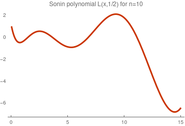
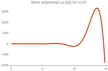
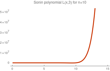
has polynomial solutions, denoted by \( L_n^{(\alpha )} (x) \) or L(α, x) and called the generalized/associated Laguerre polynomials, or Sonin polynomials, after their inventor, a Russian mathematician Nikolay Yakovlevich Sonin (1849--1915). They can be defined either by the Rodrigues formula
\begin{equation} \label{EqLaguerre.6} L_n^{(\alpha )} (x) = x^{-\alpha} \,\frac{e^x}{n!} \, \frac{{\text d}^n}{{\text d} x^n} \left( x^{n+\alpha} e^{-x} \right) = x^{-\alpha} \,\frac{1}{n!} \left( \frac{\text d}{{\text d}x} -1 \right)^n x^{n+\alpha} , \qquad n=0,1,2,\ldots ; \end{equation}
or through its ordinary generating function
\[ \frac{1}{(1-t)^{\alpha +1}} \, e^{-xt/(1-t)} = \sum_{n\ge 0}^n L_n^{(\alpha )} (x)\, t^n . \]

It can be expressed through a confluent hypergeometric function of the first kind
\[ L_n^{(\alpha )} (x) = \frac{\Gamma (n+ \alpha +1)}{n! \,\Gamma (\alpha )}\,_1F_1 \left( -n; \alpha +1; x \right) = \binom{n+\alpha}{n} \,_1F_1 \left( -n; \alpha +1; x \right) . \]
Another useful formula:
\[ L_n^{(\alpha )} (x) = \Gamma (n+ \alpha +1) \sum_{k=0}^n \frac{1}{k!\,(n-k)!\,\Gamma (k+\alpha +1)}\left( -x \right)^k . \]

Although Mathematica has a build-in command for the Sonin polynomial, LaguerreL[n, a, x], we find first five Sonin polynomials from the generating function:

Series[(1/(1-t))^(alpha) * Exp[-x*t/(1-t)]/(1-t), {t, 0, 10}]
       n     Sonin polynomial
    n = 0         L0(x; α) = 1
    n = 1         L1(α)(x; α) = 1 − x + α
    n = 2         \( \displaystyle L_2^{(\alpha )} (x) = \frac{1}{2} \left[ x^2 - \left( 2\alpha + 4 \right) x + \left( \alpha + 1 \right) \left( \alpha + 2 \right) \right] \)
    n = 3         \( \displaystyle L_3^{(\alpha )}(x) = \frac{1}{6} \left( 11\alpha +6 + 6\alpha^2 + \alpha^3 -18x -15\alpha\,x - 3 \alpha^2 x + 9 x^2 + 3\alpha x^2 - x^3 \right) \)
    n = 4         \( \displaystyle L_4^{(\alpha )} (x) = \frac{1}{24} \left[ x^4 - 4\alpha x^3 -16 x^3 + 6 \alpha^2 x^2 + 42\alpha\,x^2 + 72\,x^2 + 4\alpha^3 x -36\alpha^2 x -104 \alpha x -96\,x + \alpha^4 + 10\alpha^3 + 35\alpha^2 + 50\alpha + 24 \right] \)

They can be defined explicitly:

\[ L_n^{(\alpha )} (x) = \sum_{k=0}^n \frac{(\alpha + n)^{\underline{n-k}}}{k!\, (n-k)!}\, (-x)^k = \sum_{k=0}^n \frac{\Gamma (n + \alpha + 1)}{\Gamma (\alpha + k + 1)\,k!\, (n-k)!} \left( -x \right)^k = \sum_{k=0}^n (-1)^k \binom{n+\alpha}{n-k} \frac{x^k}{k!} , \qquad n=0,1,2,\ldots . \]

Example 2: Using Mathematica, we plot some Sonin polynomials

Plot[LaguerreL[10, 1/2. x], {x, 0, 15}, PlotTheme -> "Web", PlotLabel -> "Sonin polynomial L(x,1/2) for n=10"]
Plot[LaguerreL[10, 3/2. x], {x, 0, 15}, PlotTheme -> "Web", PlotLabel -> "Sonin polynomial L(x,3/2) for n=10"]
Plot[LaguerreL[10, 3. x], {x, 0, 15}, PlotTheme -> "Web", PlotLabel -> "Sonin polynomial L(x,3) for n=10"]
       
       
Sonin polynomial L10(1/2)(x)         Sonin polynomial L10(3/2)(x)         Sonin polynomial L10(3)(x)

Example 3: The most important application of the Laguerre polynomials is in the solution of the Schrödinger equation for the hydrogen atom. This equation is

\[ -\frac{\hbar^2}{2m}\, \nabla^2 \psi - \frac{Ze^2}{4\pi \epsilon_0 r} \, \psi = E\,\psi , \]
in which Z = 1 for hydrogen, 2 for ionized helium, and so on. Separating variables, we find that the angular dependence of ψ is the spherical harmonic \( Y_L^M \left( \theta , \varphi \right) . \) The radial part, R(r), satisfies the equation
\[ -\frac{\hbar^2}{2m}\, \frac{1}{r^2} \, \frac{\text d}{{\text d}r} \left( r^2 \frac{{\text d}R}{{\text d}r} \right) - \frac{Ze^2}{4\pi \epsilon_0 r} \, R + \frac{\hbar^2}{2m}\, \frac{L(L+1)}{r^2} \,R = E\,R . \]
For bound states, \( R \mapsto 0 \ \mbox{as } \ r \mapsto \infty , \) and R is finite at the origin r = 0. To solve this Sturm--Liouville problem, we use the abbreviations
\[ \rho = \alpha r, \qquad \alpha^2 = - \frac{8mE}{\hbar^2}, \qquad \lambda = \frac{mZe^2}{2\pi \epsilon_0 \alpha \hbar^2}, \quad E<0. \]
Then for \( \chi (\rho ) = R(\rho /\alpha ) , \) we get
\[ \frac{1}{\rho^2} \, \frac{\text d}{{\text d}\rho} \left( \rho^2 \frac{{\text d}\chi (\rho)}{{\text d}\rho} \right) + \left( \frac{\lambda}{\rho} - \frac{1}{4} - \frac{L(L+1)}{\rho^2} \right) \chi (\rho ) =0. \]
Its solution is
\[ \rho \,\chi (\rho ) = e^{-\rho^2 /2}\, \rho^{L+1}\, L_{\lambda -L-1}^{(2L+1)} (\rho ) . \]
We must restrict the parameter λ by requiring it to be an integer \( n, \ n=1,2,\ldots . \) This is necessary because the Laguerre function of nonintegral n would diverge, which is unacceptable for our physical problem, in which \( \lim_{r\to\infty} R(r) =0. \) This restriction on λ, imposed by our boundary condition, has the effect of quantifying the energy
\[ E_n = -\frac{Z^2 m}{2n^2 \hbar^2} \left( \frac{e^2}{4\pi \epsilon_0} \right)^2 . \]
The negative sign reflects the fact that we are dealing here with bound states, corresponding to an electron that is unable to escape to infinity, where the Coulomb potential goes to zero. Using this result for En, we have
\[ \alpha = \frac{m e^2}{2\pi \epsilon_0 \hbar^2} \cdot \frac{Z}{n} = \frac{2Z}{n\,a_0} , \qquad \rho = \frac{2Z}{n\,a_0} \,r , \]
with
\[ a_0 = \frac{4\pi \epsilon_0 \hbar^2}{me^2} , \qquad\mbox{the Bohr radius} . \]


Recurrences involving Sonin Polynomials


Using the generating function, the following recurrences are derived.
\[ \begin{split} \left( n+1 \right) L_{n+1}^{(\alpha )} (x) &= \left( 2n+1 + \alpha -x \right) L_n^{(\alpha )} (x) - \left( n + \alpha \right) L_{n-1}^{(\alpha )} (x) , \\ L_n^{(\alpha )} (x) &= L_n^{(\alpha +1)} (x) - L_{n-1}^{(\alpha +1)} (x) , \qquad n=1,2,\ldots . \end{split} \tag{R.4} \]
Simplify[LaguerreL[9, 3/2, x] - LaguerreL[9, 5/2, x] + LaguerreL[8, 5/2, x]]
\[ x\,L_n^{(\alpha +1)} (x) = \left( n + \alpha + 1 \right) L_n^{(\alpha )} (x) - \left( n + 1 \right) L_{n+1}^{(\alpha )} (x) , \qquad n=1,2,\ldots . n=1,2,\ldots . \tag{R.5} \]
Simplify[x*LaguerreL[9, 3/2, x] - (10 + 1/2)* LaguerreL[9, 1/2, x] + 10*LaguerreL[10, 1/2, x]]
The recurrences for derivatives are also derived from the generating function.
\[ \frac{\text d}{{\text d}x} \, L_n^{(\alpha )} (x) = - L_{n-1}^{(\alpha +1)} (x) , \qquad n=1,2,\ldots . \tag{R.6} \]
Simplify[D[LaguerreL[9, 3/2, x] , x] + LaguerreL[8, 5/2, x]]
\[ x\,\frac{\text d}{{\text d}x} \, L_n^{(\alpha )} (x) = n\,L_n^{(\alpha )} (x) - \left( n+ \alpha \right) L_{n-1}^{(\alpha )} (x) . n=1,2,\ldots . \tag{R.7} \]
Simplify[x*D[LaguerreL[9, 3/2, x] , x] + (9 + 3/2)* LaguerreL[8, 3/2, x] - 9*LaguerreL[9, 3/2, x]]
\[ L_n^{(\alpha +1)} (x) = \sum_{\nu =0}^n L_{\nu}^{(\alpha )} (x) . \tag{R.8} \]
Simplify[Sum[LaguerreL[k, 3/2, x], {k, 0, 7} ] - LaguerreL[7, 5/2, x]]

The Sonin polynomial can be expressed through Laguerre polynomials:

\[ L_n^{(\alpha +1)} (x) = \sum_{k =0}^n \binom{\alpha + k -1}{k} L_{k} (x) . \tag{R.9} \]
Simplify[Sum[LaguerreL[5-k, x]*Binomial[k+1/2,k], {k, 0, 5} ] - LaguerreL[5,3/2,x]]

Suppose that for α > −1, a real-valued function f(x), defined on the half-line (0, ∞) has a finite integral

\[ \| f \|^2 = \langle\, f, f\,\rangle_w = \int_0^{\infty} \frac{x^{\alpha} e^{-x}}{\Gamma (\alpha +1)} \left\vert f(x) \right\vert^2 {\text d} x < \infty , \qquad \alpha > -1. \]
Then this function can be expanded into the (formal) Sonin series
\begin{equation} \label{EqLaguerre.7} f(x) = \sum_{n\ge 0} f_i^{(\alpha )} L_i^{(\alpha )} (x) , \qquad f_i^{(\alpha )} = \frac{1}{\Gamma (\alpha +1)} \int_0^{\infty} f(x)\,L_i^{(\alpha )} (x) \,x^{\alpha} e^{-x} {\text d} x , \quad i=0,1,2,\ldots . \end{equation}

Since a set of Sonin polynomials { Ln(α, x) }n∈ℕ form a complete orthogonal system in the Hilbert space 𝔏²(ℝ, xαe−x), the coefficients fi of expansion \eqref{EqLaguerre.7} satisfy Parseval's identity (it can be extended for complex-values functions):

\[ \| f \|^2 = \frac{1}{\Gamma (\alpha +1)} \int_0^{\infty} f^2 (x)\, x^{\alpha} e^{-x} {\text d} x = \sum_{n\ge 0} \binom{i+\alpha}{i} \left\vert f_i^{(\alpha )} \right\vert^2 . \]


Some Useful Formulas


The Sonin polynomials satisfy the orthogonality property
\[ \int_0^{\infty} L_n^{(\alpha )} (x)\,L_m^{(\alpha )} (x)\, x^{\alpha} e^{-x} {\text d} x = \frac{\Gamma (n + \alpha + 1)}{\Gamma (n+1)}\,\delta_{n,m} , \]
where δn,m is the Kroneker delta. The initial data are
\[ L_n^{(\alpha )} (0) = \frac{\Gamma (n + \alpha + 1)}{\Gamma (n + 1)\, \Gamma (\alpha + 1)} = \binom{n+\alpha}{n} , \qquad \left( \frac{\text d}{{\text d} x}\, L_n^{(\alpha )} (x) \right)_{x=0} = - \binom{n+\alpha}{n-1} . \]

Sonin's polynomials can be expressed through the Bessel function of the first kind:

\[ L_n^{(\alpha )} (x) = \frac{1}{n!}\, e^x x^{-\alpha /s} \int_0^{\infty} t^{n+ \alpha /s} J_{\alpha} \left( 2\sqrt{xt} \right) e^{-t} {\text d}t . \]

Theorem 2: The Laplace transform of the Sonin polynomial is
\[ {\cal L}_{x\to \lambda} \left[ L_n^{(\alpha )} (x) \right] = \int_0^{\infty} L_n^{(\alpha )} (x)\, e^{-\lambda x}{\text d} x = \binom{n+\alpha}{n} \,\frac{(\lambda -1)^{\alpha +n}}{\lambda^{1+n+\alpha}}\,_2F_1 \left( \alpha , 1 + \alpha +n , \alpha +1; \frac{1}{\lambda} \right) = \frac{1}{\lambda} \sum_{k=0}^n \binom{\alpha + k-1}{k} \left( 1 - \frac{1}{\lambda} \right)^{n-k} . \]
where 2F1 is the hypergeometric function.
Let Y(λ) be the Laplace transform of the Sonin polynomial:
\[ Y(\lambda ) = {\cal L}_{x\to \lambda} \left[ y(x) \right] = \int_0^{\infty} y(x)\, e^{-\lambda x} {\text d} x = \int_0^{\infty} L_n^{(\alpha )} (x)\, e^{-\lambda x} {\text d} x , \tag{S.1} \]
where \( \displaystyle y(x) = L_n^{(\alpha )} (x) \) is the Sonin polynomial of degree n. Applying the Laplace transformation to the Sonin equation \eqref{EqLaguerre.5}, we obtain
\[ \left( \lambda - \lambda^2 \right) \frac{{\text d}Y(\lambda )}{{\text d}\lambda} + \left( \alpha \lambda + n +1 - \lambda \right) Y(\lambda ) = \alpha\, y(0) . \tag{S.2} \]

Note that the fiirst order differential equation (S.2) has two singular points λ = 0 and λ = 1. It contains only one initial condition because the Sonin equation has a regular singular point at the origin. To solve Eq.(S.2), we apply Bernoulli's method (see Part II,xiii of the first tutorial); so we seek its solution as the product Y = uv, where u(λ) is a solution of the homogeneous equation

\[ \left( \lambda - \lambda^2 \right) \frac{{\text d}u(\lambda )}{{\text d}\lambda} + \left( \alpha \lambda + n +1 - \lambda \right) u(\lambda ) = 0 . \tag{S.3} \]
Integrate[(1 + n + a*s - s)/s/(1 - s), s]
-(a + n) Log[1 - s] + (1 + n) Log[s]
This yields
\[ u(\lambda ) = \frac{(\lambda -1)^{\alpha +n}}{\lambda^{1+n}} . \tag{S.4} \]
Then v(λ) becomes a solution of a separable equation
\[ u\left( \lambda - \lambda^2 \right) \frac{{\text d}v(\lambda )}{{\text d}\lambda} = \alpha\,y(0) . \tag{S.5} \]
Again, separating variables and using the expression \( \displaystyle u(\lambda )\left( \lambda - \lambda^2 \right) = -\frac{( \lambda -1)^{\alpha +n+1}}{\lambda^{n}} , \) we get
\[ v' = \alpha\,y(0) \,\frac{1}{u(\lambda )\left( \lambda - \lambda^2 \right)} \qquad \Longrightarrow \qquad v(\lambda ) = \alpha\,y(0) \,\frac{1}{\alpha \lambda^{\alpha}}\,_2F_1 \left( a, 1 + \alpha +n. \alpha +1; \frac{1}{\lambda} \right) , \tag{S.6} \]
where 2F1 is the hypergeometric function.
Integrate[s^n /(1 - s)^(1 + n + a), s]
(s^(1 + n) Hypergeometric2F1[1 + n, 1 + a + n, 2 + n, s])/(1 + n)
Multiplying these functions and using the initial condition y(0), we obtain the Laplace transform of the Sonin polynomial:
\[ Y(\lambda ) = \binom{n+\alpha}{n} \,\frac{(\lambda -1)^{\alpha +n}}{\lambda^{1+n+\alpha}}\,_2F_1 \left( \alpha , 1 + \alpha +n , \alpha +1; \frac{1}{\lambda} \right) . \]
We check some values with Mathematica.

For n = 0, we have L(0, x) = 1,

FullSimplify[Binomial[n + a, n]*(s - 1)^(a + n)/s^(1 + n + a) * Hypergeometric2F1[a, 1 + a + n, a + 1, 1/s] /. n -> 0]
1/s
For n = 1, we have L(0, x) = 1 −x + α,
FullSimplify[ Binomial[n + a, n]*(s - 1)^(a + n)/s^(1 + n + a) * Hypergeometric2F1[a, 1 + a + n, a + 1, 1/s] /. n -> 1]
(-1 + s + a s)/s^2
LaplaceTransform[LaguerreL[1, a, x], x, s]
-(1/s^2) + 1/s + a/s
﹡ ⁎ ✱ ✲ ✳ ✺ ✻ ✼ ✽ ❋
From this theorem, one can derive
\[ {\cal L}_{x\to\lambda} \left[ x^{\alpha} L_n^{(\alpha )} (x) \right] = \frac{\Gamma (n+\alpha +1)}{n!\,\lambda^{\alpha +1}} \left( 1 - \frac{1}{\lambda} \right)^n , \]
and
\[ {\cal L}_{x\to\lambda} \left[ x^p L_n (x) \right] = \frac{\Gamma (p+1)}{\lambda^{p+n+1}} \sum_{k=1}^n \left( -1 \right)^k \binom{n}{k} \binom{p}{k} \left( \lambda -1 \right)^{n-k} . \]


Connection with Hermite Polynomials


The Hermite polynomial satisfy the relations:
\[ H_{2k} (x) = (-1)^k 4^k k!\, L_k^{(-1/2 )} (x^2 ) ; \]
\[ H_{2k+1} (x) = (-1)^k 4^k k!\, L_k^{(1/2 )} (x^2 ) . \]

Correspondingly, the reverse relations are valid:

\[ L_n^{(-1/2 )} (x) = \frac{(-1)^n}{n!\, 4^n}\, H_{2n} \left( \sqrt{x} \right) , \qquad n=0,1,2,\ldots ; \]
\[ L_n^{(1/2 )} (x) = \frac{(-1)^n}{n!\, 2^{2n+1} \sqrt{x}}\, H_{2n+1} \left( \sqrt{x} \right) , \qquad n=0,1,2,\ldots . \]

If α > −½, then the Sonin polynomials can be expressed in terms of H2k as follows

\[ L_n^{(\alpha )} (x) = \frac{(-1)^n}{\Gamma \left( \alpha + \frac{1}{2} \right) \sqrt{\pi}} \cdot \frac{\Gamma (n+ \alpha +1)}{(2n)!} \int_{-1}^1 \left( 1 - t^2 \right)^{\alpha -1/2} H_{2n} \left( t\sqrt{x} \right) {\text d}t . \]
  1. Barrera-Figueroa, V., Guerrero-Moreno, I., López-Bonilla, J., Laguerre, E., Laplace Transform of Laguerre Associated Polynomial, Prespacetime Journal, January2017, Volume 8, Issue 1, pp. 80--83.
  2. Chebyshev, P., L. "Sur le développement des fonctions à une seule variable." Bull. Ph.-Math., Acad. Imp. Sc. St. Pétersbourg 1, 193-200, 1859.
  3. Chebyshev, P. L. Oeuvres, Vol. 1. New York: Chelsea, pp. 499-508, 1987.
  4. Hassani, M.E., A note on Laguerre original ODE and Polynomials (1879), Institute for Fundamental Research, 2020.
  5. Laguerre, E. de. Sur le transformations des fonctions elliptiques, Bulletin de la Société Mathématique de France, 1878, 6, 72–78
  6. Laguerre, E. de. Sur l'intégrale int_x^(+infty)x^(-1)e^(-x)dx," Bulletin de la Société Mathématique de France, 1879, 7, pp. 72--81. Reprinted in Oeuvres, Vol. 1. New York: Chelsea, pp. 428-437, 1971.
  7. Sonine, N. J. "Sur les fonctions cylindriques et le développement des fonctions continues en séries." Math. Ann. 16, 1-80, 1880.
  8. Szegö, G. Orthogonal Polynomials, 4th ed. Providence, RI: Amer. Math. Soc., 1975.
  9. Terekhov, A.V., Generating the Laguerre expansion coefficients by solving a one-dimensional transport equation,


Return to Mathematica page
Return to the main page (APMA0340)
Return to the Part 1 Matrix Algebra
Return to the Part 2 Linear Systems of Ordinary Differential Equations
Return to the Part 3 Non-linear Systems of Ordinary Differential Equations
Return to the Part 4 Numerical Methods
Return to the Part 5 Fourier Series
Return to the Part 6 Partial Differential Equations
Return to the Part 7 Special Functions