This section gives an introduction to nonlinear one dimensional oscilaltors.
We consider only unforced models leaving driven cases to other sections.
Such models turns up in a wide variaty of physical problems and play a major
and vital role in the analysis of such systems.
Our approach is to demonstrate applications of software in the description of
many examples and case studies.
Return to computing page for the first course APMA0330
Return to computing page for the second course APMA0340
Return to Mathematica tutorial for the first course APMA0330
Return to Mathematica tutorial for the second course APMA0340
Return to the main page for the first course APMA0330
Return to the main page for the second course APMA0340
Return to Part III of the course APMA0340
Introduction to Linear Algebra with Mathematica
An oscillator is a physical system characterized by periodic motion, such as a
spring-mass system, which is a classic example of harmonic oscillation when
the restoring force is proportional to the displacement.
Anharmonic oscillators, however, are characterized by the nonlinear dependence
of the restorative force on the displacement. Consequently, the anharmonic
oscillator's period of oscillation may depend on its amplitude of oscillation.
There are many systems throughout the physical world that can be modeled as
anharmonic oscillators in addition to the nonlinear mass-spring system.
In quantum mechanics, an oscillator is described by the
Schrödinger equation
where j is the imaginary unit so j² = -1,
ℏ = h/(2 π) is the reduced Planck constant, h ≈ 6.626068 × 10⁻³⁴ m² kg/s is Planck's constant, an incredibly small number named after the physicist Max Planck who had already guessed this formula in 1900 in his work on black body radiation, and Ψ (the Greek letter
psi) is the state vector of the quantum system, t is time, and
H is the Hamiltonian operator.
The most famous example is the nonrelativistic Schrödinger equation for the
wave function in position space of a single particle subject to a potential
V, such as that due to an electric field
where m is the particle's mass, ∇² is the Laplacian, and V
is the potential energy of the particle (a function of x, y,
z, and t).
However, the equation can be separated into temporal and spatial parts (when
V is independent of time) using
separation of variable \( \Psi (x,t) = \psi (x)\, T(t) \)
to obtain
the time-independent Schrödinger equation
A usual spring-mass system is governed by Newton's second law:
\[
m\,\ddot{x} = f(x) ,
\]
where m is the particle's mass of a weight attached to
the spring, x(t) is the displacement from the equilibrium
position, and f(t) represents the restoring force.
It is useful to introduce "natural units" for length and energy in order the
time independent Schrödinger equation and spring-mass equation to be reduced
to dimensionless form, which can be written as
\[
\ddot{x} = f(x) .
\]
In dissipative systems, the restoring force may depend also on the derivative
\( \dot{x} . \) Since the restoring force can be
considered as the derivative of the potential energy, the anharmonic equation
in reduced units becomes
where \( \ddot{x} = {\text d}^2 x/{\text d} t^2 \)
is the second derivative with respect to time variable.
The potential energy function of a one-dimensional oscillator about its stable
equilibrium position, which we take to be x = 0, can usually be
expanded in a Taylor series:
where V0 is the value of V(x) at the
equilibrium point, and \( V_0^{(n)} \) is the
n-th order derivative of the potential function evaluated at that point.
The constant term V0 can be set equal to zero without loss
of generality because the potential energy is only defined to within an
additive constant. Furthermore, the coefficient of the first order term
vanishes since at the equilibrium point, the potential energy function has a
local minimum. Consequently, the power series expansion will be
In order for the potential energy to have local minimum at x = 0, the
second order term cannot be negative, \( V_0^{(2)} > 0.
\) Multiplying the differential equation
\( \ddot{x} + \frac{\partial V}{\partial x} =0 \)
by \( \dot{x} , \) we obtain
the total energy. In many cases, the potential function V(x) can
be represented or approximated by a polynomial; however, in some cases it is
not the case.
We start by considering one particular anharmonic motion from music, when two
real tones are
sounded at the same time. In addition to these two tones, one can hear an
auxiliary tone or tones that are artificially perceived when two real tones
are sounded at the same time. Their discovery is credited to the violinist
Giuseppe Tartini
(although it was first discovered by the organist George Sorge in about 1745) and so are also
called Tartini tones. This effect is most often used in the lowest
octave of the organ only. It can vary from highly effective to disappointing
depending on several factors, primarily the skill of the organ voicer, and the
acoustics of the room the instrument is installed in.
The subjective existence of these combination tones was first investigated
theoretically by the German physician and physicist Hermann von Helmholtz (1821--1894). He concluded that the transient displacement x
of the tympanic membrane of the ear from its equilibrium position in response
to some imposed vibration is governed by the equation
where ω²0 = k/m is the natural frequency
of the ear drum and α is a parameter associated with the nonlinear
response of the ear drum
to the imposed vibration. This equation is often referred to as the
anharmonic motion equation as it has subsequently been employed for
describing the nonlinear anharmonic oscillations. The initial value problem
consisting of the anharmonic equation and usual initial conditions
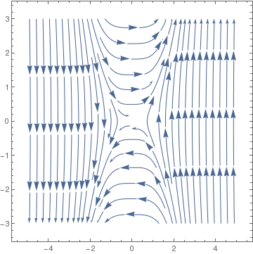
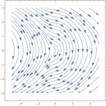
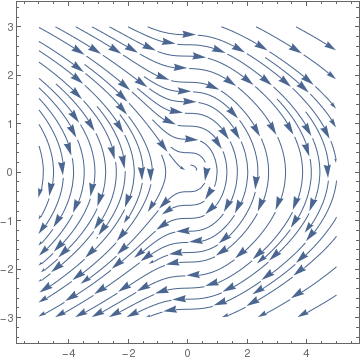
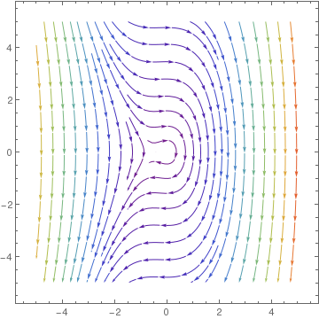
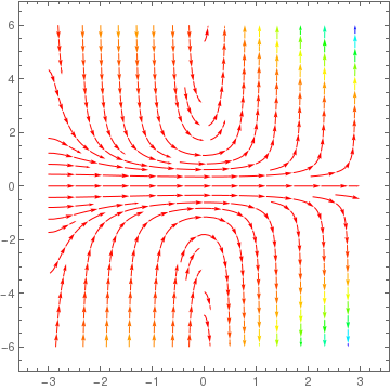
has two equilibrium solutions: the origin is a center, and
\( \left( -1/\varepsilon , 0 \right) \)
is a saddle point (subject to ϵ ≠ 0). We plot phase
portraits for different values of ϵ:
To find its energy
integral, we multiply the equation by \( \dot{x} =
{\text d}x/{\text d}t \) and integrate with respect to time variable.
This yields
Example:
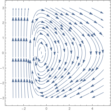
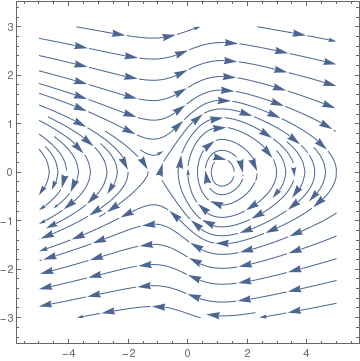
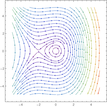
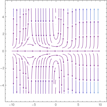
Consider the mass-spring equation \( \ddot{x} + x - x^2 /2
=0 , \) which can be reduced to the following system of first order
differential equations
This system has the two equilibrium solutions: a center at the
origin and a saddle point at (2,0). The separatrix is a
trajectory that passes through the saddle point.
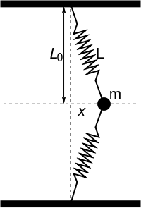
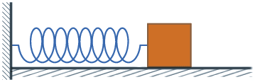
Consider a particle of mass m, tethered symmetrically by two identical springs that can oscillate along the x axis, as shown in Figure. Each spring is assumed to satisfy Hooke's law with a constant k ans a relaxed for outstretched length ℓ0. The gravitational force is either absent or balanced by some other sources, so that the springs are the only sources of force on the particle. When the particle is at position x, the potential energy of the system is
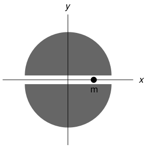
Consider a sphere of radius R with a nonuniform, but radially
symmetric mass distribution given by the density function
\( \rho = \rho_0 (r/R)^s , \) where
ρ0 is a positive constant and s > -2 (not necessarily
an integer).
For a particle of mass m, located at a distance r ≤ R
from the center of the mass distribution, the gravitational potential energy
of the system is given by
where M is the total mass of the sphere, which is related to the other
parameters by \( M = (4\pi \rho_0 R^3)/(s+3) . \)
If we choose the x axis so that it passes through the center of the mass distribution with its origin at that point, then along this axis is
r = |x|, and
Now suppose we dig a narrow tunnel along the x axis and release the
particle from the rest somewhere on the x axis in this tunnel. Simple
harmonic oscillations are possible when x = 0, that is, when the mass
distribution is uniform (which is not true for the Earth). In this unrealistic
case the potential energy reduces to
Example:
Consider a particle (or bead) of mass m sliding without friction on a
curve (or wire) is a vertical plane (the xy plane), with a minimum at
x = 0. The curve can have any profile y = f(x)
because a wire can be arbitrary in shape. However, we consider two simple
cases when \( y = c\, x^2 \) or
\( y = c\, x^4 \) for some positive constant
c.
The potential energy will be
\[
\Pi (s) = mg\, y = mg\,c\, s^2 \qquad \mbox{or} \qquad \Pi (s) = mg\, c\, s^4 .
\]
Then the total energy becomes
\[
E = \frac{1}{2}\, m\,\dot{s}^2 + mg\,c\, s^n , \qquad \mbox{where} \quad
n = 2,4.
\]
Example:
The Morse potential, named after physicist Philip M. Morse (1903--1985), is a convenient interatomic interaction model for the potential energy of a diatomic molecule. It is a better approximation for the vibrational structure of the molecule than the QHO (quantum harmonic oscillator) because it explicitly includes the effects of bond breaking, such as the existence of unbound states. The celebrated Morse potential (1929) is described by the two-parameter function
This potential attains minimum at the origin, with a well depth V0 and scale parameter k. For a particle with mass m0, we introduce the dimensionless length and energy variables
Phase portrait for the Morse potential
A simple change of variable \( \rho = \sqrt{2K}\, e^{-u/2}
\) transfers the Schrödinger equation into the radial equation of a two-dimensional harmonic oscillator with unit mass and unit angular frequency:
Example:
A Pöschl–Teller potential, named after the physicists Herta Pöschl (credited as G. Pöschl) and Edward Teller, is a special class of potentials for which the one-dimensional Schrödinger equation can be solved in terms of special functions. Herta and Edward, while being at Göttingen university, discovered this potential in 1932. After the Nazis came to power in 1933, conditions for Jews in Germany rapidly deteriorated and Teller left the country first to Copenhagen and then to London. In 1935, Teller was recruited at George Washington University, in Washington, D.C. The Pöschl–Teller potential can be defined as
\[
V(x) = - \frac{V_0}{\cosh^2 (kx)} .
\]
So the Schrödinger equation with Pöschl–Teller potential becomes
Phase portrait for the Schrödinger equation with Pöschl–Teller potential
The solutions of this time-independent Schrödinger equation
can be found by virtue of the substitution u = tanh(x),
which yields the Legendre equation.
■
The Rosen--Morse potential was originally proposed as an analytical model to study the energy levels of the NH3 molecule.
■
Example:
The hydrogen atom, consisting of an electron and a proton, is a two-particle system, and the internal motion of two particles around their center of mass is equivalent to the motion of a single particle with a reduced mass. This reduced particle is located at r, where r is the vector specifying the position of the electron relative to the position of the proton. The length of r is the distance between the proton and the electron, and the direction of r and the direction of r is given by the orientation of the vector pointing from the proton to the electron. Since the proton is much more massive than the electron, we will assume that the reduced mass equals the electron mass and the proton is located at the center of mass.
The hydrogen atom Hamiltonian also contains a potential energy term, V, to describe the attraction between the proton and the electron. This term is the Coulomb potential energy
\[
V(r) = - \frac{e^2}{4\pi \epsilon_0 r} ,
\]
where r is the distance between the electron and the proton. The Coulomb potential energy depends inversely on the distance between the electron and the nucleus and does not depend on any angles. Such a potential is called a central potential.
The time-independent Schrödinger equation (in spherical coordinates) for a electron around a positively charged nucleus is then
Using Bohr's radius \( a = \hbar^2 /me^2 \) and the hydrogen ionization energy \( {\cal E} = m\.e^4 /2\hbar^2 \) as unit length and unit energy, it is possible to recast the above equation as
Gatland, I.R., Theory of a nonharmonic oscillator, American Journal of
Physics, 1991, Vol. 59, No. 2, pp. 155--158; doi: 10.1119/1.16597
Kim Johannessen, An anharmonic solution to the equation of motion for the
simple pendulum, European Journal of Physics, 2011, Vol. 32, No. 2, pp.407-- doi: 10.1088/0143-0807/32/2/014
Mohazzabi, P., Theory and examples of intrinsically nonlinear oscillators,
American Journal of Physics, 2004, Vol. 72, No. 4, pp. 492--498;
doi: https://doi.org/10.1119/1.1624114
Peters, J.M., Bulletin of the Institute of Mathematics and its
Applications, 1981, Vol. 17,
Usher, J.R. and Nye, V.A., Further observations on the anharmonic motion
equation, International Journal of Mathematical Education in Science and Technology, 1989, Vol. 20, No 3, pp. 399--406; doi: 10.1080/00207398902000308
Return to Mathematica page
Return to the main page (APMA0340)
Return to the Part 1 Matrix Algebra
Return to the Part 2 Linear Systems of Ordinary Differential Equations
Return to the Part 3 Non-linear Systems of Ordinary Differential Equations
Return to the Part 4 Numerical Methods
Return to the Part 5 Fourier Series
Return to the Part 6 Partial Differential Equations
Return to the Part 7 Special Functions
 An oscillator is a physical system characterized by periodic motion, such as a
spring-mass system, which is a classic example of harmonic oscillation when
the restoring force is proportional to the displacement.
Anharmonic oscillators, however, are characterized by the nonlinear dependence
of the restorative force on the displacement. Consequently, the anharmonic
oscillator's period of oscillation may depend on its amplitude of oscillation.
An oscillator is a physical system characterized by periodic motion, such as a
spring-mass system, which is a classic example of harmonic oscillation when
the restoring force is proportional to the displacement.
Anharmonic oscillators, however, are characterized by the nonlinear dependence
of the restorative force on the displacement. Consequently, the anharmonic
oscillator's period of oscillation may depend on its amplitude of oscillation.
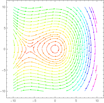
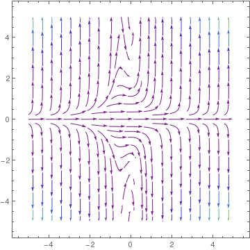
 Then we use negative ε: -1.5, -1, -200/19, -10/9.
■
Then we use negative ε: -1.5, -1, -200/19, -10/9.
■