Return to computing page for the first course APMA0330
Return to computing page for the second course APMA0340
Return to computing page for the fourth course APMA0360
Return to Mathematica tutorial for the first course APMA0330
Return to Mathematica tutorial for the second course APMA0340
Return to Mathematica tutorial for the fourth course APMA0360
Return to the main page for the first course APMA0330
Return to the main page for the second course APMA0340
Return to the main page for the fourth course APMA0360
Return to Part V of the course APMA0340
Introduction to Linear Algebra with Mathematica
This section is a collection of Fourier series expansions for different
functions.
Theorem: If a periodic function of period \( 2\ell \) is
square-integrable on any finite interval, then the Fourier series converges to the function at almost every point:
\[
f(x) \,\sim \, \frac{a_0}{2} + \sum_{k\ge 0} \left[ a_k \cos \left( \frac{k \pi x}{\ell} \right) + b_k \sin \left( \frac{k \pi x}{\ell} \right) \right] ,
\]
where its coefficients are determined via Euler--Fourier formula:
\[
\begin{split} a_k &= \frac{1}{\ell} \, \int_{-\ell}^{\ell} f(x)\,\cos \left( \frac{k \pi x}{\ell} \right) {\text d} x , \quad k=0,1,2,\ldots ,
\\
b_k &= \frac{1}{\ell} \, \int_{-\ell}^{\ell} f(x)\,\sin \left( \frac{k \pi x}{\ell} \right) {\text d} x , \quad k=1,2,\ldots .
\end{split} \qquad\qquad ■
\]
Expansion in a
complex form (or exponential form):
\begin{equation} \label{EqFourier.1}
f(x) \,\sim\, \mbox{P.V.}\sum_{n=-\infty}^{\infty} \hat{f}(n)\, e^{n{\bf j} \pi x/\ell} = \lim_{N\to \infty} \sum_{n=-N}^{N} \hat{f}(n)\, e^{n{\bf j} \pi x/\ell} ,
\end{equation}
where
T = 2ℓ is the period and the Fourier coefficients
\( \hat{f}(n) \) are evaluated according to the Euler--Fourier formula:
\begin{equation} \label{EqFourier.2}
\hat{f}(n) = \frac{1}{2\ell} \int_{-\ell}^{\ell} f(x)\, e^{-n{\bf j} \pi x/\ell} \,{\text d} x = \frac{1}{T} \int_{0}^{T} f(x)\, e^{-2n{\bf j} \pi x/T} \,{\text d} x , \qquad n \in \mathbb{Z} = \left\{ 0, \pm 1, \pm 2, \ldots \right\} .
\end{equation}
Here «P.V.» abbreviates the
Cauchy principle value, which is a regularization of the infinite sum.
The first examples are based on well-known sum of geometric series
\[
\frac{1}{2} + z + z^2 + z^3 + \cdots = \frac{1}{2} \cdot \frac{1+z}{1-z} ,
\]
where
\( z = r\,e^{{\bf j}x} . \) Extraction of real and imaginary parts yields the following series:
\[
P(r, x) = \frac{1}{2} + \sum_{n\ge 1} r^n \cos (nx) = \mbox{P.V.} \sum_{n = -\infty}^{\infty} r^{|n|} e^{{\bf j}nx} = \frac{1}{2} \cdot \frac{1 + r^2}{1- 2r\,\cos x + r^2} ,
\]
\[
Q(r, x) =\sum_{n\ge 1} r^n \sin (nx) = \frac{1}{2} \cdot \frac{r\, \sin x}{1- 2r\,\cos x + r^2} .
\]
The function
P(
r, x) is called the
Poisson kernel.
Similarly, from the formula
\[
\ln \frac{1}{1-z} = z + \frac{1}{2}\, z^2 + \frac{1}{3}\, z^3 + \frac{1}{4}\, z^4 + \cdots \qquad (0 \le r < 1),
\]
we get
\[
\sum_{n\ge 1} \frac{\cos nx}{n}\,r^n = \frac{1}{2} \cdot \ln \frac{1}{1 - 2r\,\cos x + r^2} , \qquad \sum_{n\ge 1} \frac{\sin nx}{n}\, r^n = \arctan \frac{r\,\sin x}{1 - 2r\,\cos x + r^2} .
\]
From these sums, we derive
\begin{eqnarray*}
\sum_{n\ge 1} \frac{1}{n} \, \cos n x &=& -\frac{1}{2} \, \ln \left[ 2 \left( 1 - \cos x \right) \right] , \qquad \mbox{on interval } \ 0 < x < 2\pi ;
\\
\sum_{n\ge 1} \frac{1}{n} \, \sin n x &=& \begin{cases}
\phantom{-}\frac{\pi -x}{2} , & \ \mbox{for } 0< x < \pi , \\
- \frac{\pi +x}{2} , & \ \mbox{for } -\pi < x < 0 ,
\end{cases} \qquad \mbox{on interval } \ -\pi < x < \pi .
\\
\sum_{n\ge 1} \frac{1}{n} \, \sin \frac{n\pi x}{\ell} &=& \frac{\ell-x}{2}
, \qquad 0 < x < 2\ell .
\\
\sum_{n\ge 1} \frac{(-1)^{n+1}}{n} \, \cos n x &=& \ln \left( 2 \, \cos \frac{x}{2} \right) , \qquad \mbox{on interval } \ |x| < \pi ;
\\
\sum_{n\ge 1} \frac{(-1)^{n+1}}{n} \, \sin n x &=& \frac{x}{2} , \qquad \mbox{on interval } \ |x| < \pi .
\end{eqnarray*}
\[
\frac{1}{2{\bf j}}\,\sum_{n\ne 0} \frac{e^{{\bf j}nx}}{n} = \begin{cases}
- \frac{\pi}{2} - \frac{x}{2} , & \ \mbox{ if} \quad -\pi < x < 0 ,
\\ 0 , & \ \mbox{ if} \quad x = 0,
\\
\frac{\pi}{2} - \frac{x}{2} , & \ \mbox{ if} \quad 0 < x < \pi .
\end{cases}
\]
S1[x_] = Sum[1/n*Cos[n*x] , {n, 1, 100}];
p1 = Plot[{S1[t]}, {t, 0, 2*\[Pi]},
PlotStyle -> {Thickness[0.01], Orange}];
p2 = Plot[{ -1/2 Log[2*(1 - Cos[t])]}, {t, 0, 2*\[Pi]},
PlotStyle -> {Thickness[0.007], Plue}];
Show[p1, p2]
S2[x_] = Sum[1/n*Sin[n*x], {n, 1, 100}];
Plot[{S2[t],
Piecewise[{{(\[Pi] - t)/2, 0 < t < \[Pi]}, {-(\[Pi] + t)/
2, -\[Pi] < t < 0}}]}, {t, -\[Pi], \[Pi]},
PlotStyle -> Thickness[0.01]]
S3[x_] = Sum[1/n*Sin[(n*\[Pi]*x)/l], {n, 1, 100}];
Manipulate[
Plot[{S3[t], (l - t)/2}, {t, 0, 20},
PlotStyle -> Thickness[0.01]], {l, 0, 20, Appearance -> "Labeled"}]
S4[x_] = Sum[(-1)^(n + 1)/n*Cos[n*x], {n, 1, 100}];
p41 = Plot[{S4[t], Log[2*Cos[t/2]]}, {t, -\[Pi], \[Pi]},
PlotStyle -> {Thickness[0.02], Blue}];
p42 = Plot[{S4[t], Log[2*Cos[t/2]]}, {t, -\[Pi], \[Pi]},
PlotStyle -> Thickness[0.007]];
Show[p41, p42]
S6[x_] = 1/(2 \[ImaginaryJ]) Sum[E^(\[ImaginaryJ]*n*x)/n, {n, 1, 100}];
p61 = Plot[
Piecewise[{{(-\[Pi] - t)/2, -\[Pi] < t < 0}, {0,
t = 0}, {(\[Pi] - t)/2, 0 < t < \[Pi]}}], {t, -\[Pi], \[Pi]},
PlotStyle -> {Thickness[0.01], Blue}];
p62 = Plot[{S6[t]}, {t, -\[Pi], \[Pi]},
PlotStyle -> {Thickness[0.02], Orange}];
Show[p61, p62]
\begin{eqnarray*}
\sum_{n\ge 1} \frac{1}{2n-1} \, \cos (2n-1) x &=& \frac{1}{2} \cdot \ln \left( \cot \frac{x}{2} \right) ,
\qquad \mbox{on interval } \ 0 < x < \pi .
\\
\sum_{n\ge 1} \frac{1}{2n-1} \, \sin (2n-1) x &=& \frac{1}{2} \sum_{\nu =-\infty}^{+\infty} \frac{e^{{\bf j}\left( 2\nu -1 \right) x}}{{\bf j} \left( 2\nu -1 \right)} = \frac{\pi}{4} \cdot \mbox{sign} (x) = \frac{\pi}{4} \times \begin{cases}
\phantom{-}1 , & \ \mbox{for } 0< x , \\
- 1 , & \ \mbox{for } x<0 ,
\end{cases} \qquad \mbox{on interval } \ -\pi < x < \pi .
\\
\frac{4}{\pi}\,\sum_{n\ge 1} \frac{1}{2n-1} \, \sin \frac{(2n-1)\pi x}{\ell} &=& 2 \left[ H\left( \frac{x}{\ell} \right) - H\left( \frac{x}{\ell} -1 \right) \right] -1 .
\\
\sum_{n\ge 1} \frac{(-1)^{n+1}}{2n-1} \, \cos (2n-1) x &=&
\begin{cases}
\phantom{-}\frac{\pi}{4} , & \ \mbox{for } |x|< \frac{\pi}{2} , \\
-\frac{\pi}{4} , & \ \mbox{for } |x|> \frac{\pi}{2} ,
\end{cases} \qquad \mbox{on interval } \ -\pi < x < \pi .
\\
\sum_{n\ge 1} \frac{(-1)^{n+1}}{2n-1} \, \sin (2n-1) x &=& \frac{1}{2} \,\ln \left\vert \cot \left( \frac{x}{2} - \frac{\pi}{4} \right) \right\vert , \qquad \mbox{on interval } \ -\pi < x < \pi .
\end{eqnarray*}
S7[x_] = Sum[1/(2*n - 1)*Cos[(2*n - 1)*x], {n, 1, 100}];
p71 = Plot[{S7[t]}, {t, 0, \[Pi]},
PlotStyle -> {Thickness[0.02], Purple}];
p72 = Plot[{1/2*Log[Cot[t/2]]}, {t, 0, \[Pi]},
PlotStyle -> {Thickness[0.01], Green}];
Show[p71, p72]
S8[x_] = Sum[1/(2*n - 1)*Sin[(2*n - 1)*x], {n, 1, 100}];
S81 = Plot[\[Pi]/4*Sign[t], {t, -\[Pi], \[Pi]},
PlotStyle -> {Thickness[0.007], Blue}];
S82 = Plot[{S8[t]}, {t, -\[Pi], \[Pi]},
PlotStyle -> {Thickness[0.007], Orange}];
Show[S82, S81]
Manipulate[
Plot[{4/\[Pi]*Sum[Sin[((2 n - 1)*\[Pi]*t)/l]/(2*n - 1), {n, 1, 100}],
2*(HeavisideTheta[t/l] - HeavisideTheta[t/l - 1]) - 1}, {t, -10,
10}, PlotStyle -> {{Thickness[0.01], Orange}, {Thickness[0.01],
Blue}}], {l, 1, 5}]
S10[x_] = Sum[(-1)^(n + 1)/(2 n - 1)*Cos[(2 n - 1)*x], {n, 1, 100}];
p101 = Plot[S10[t], {t, -\[Pi], \[Pi]},
PlotStyle -> {Thickness[0.015], Orange}];
p102 = Plot[{Piecewise[{{\[Pi]/4, Abs[t] < \[Pi]/2}, {-\[Pi]/4,
Abs[t] > \[Pi]/2}}]}, {t, -\[Pi], \[Pi]},
PlotStyle -> {Thickness[0.007], Blue}];
Show[p101, p102]
S11[x_] = Sum[(-1)^(n + 1)/(2 n - 1)*Sin[(2 n - 1)*x], {n, 1, 100}];
p111 = Plot[{S11[t]}, {t, -\[Pi], \[Pi]},
PlotStyle -> {Thickness[0.02], Purple}];
p112 = Plot[Log[Cot[t/2 - Pi/4]]/2, {t, -\[Pi], \[Pi]},
PlotStyle -> {Thickness[0.007], Blue}];
Show[p111, p112]
\begin{eqnarray*}
\frac{1}{2} + \sum_{n\ge 0} \frac{(-1)^n}{1+n^2} \left( \cos nx -n\,\sin nx \right) &=& \frac{\pi}{2\,\sinh \pi}\, e^x , \qquad \mbox{on interval } \ |x|< \pi .
\\
\frac{2}{\pi} - \frac{4}{\pi} \,\sum_{n\ge 1} \frac{1}{4n^2 -1} \, \cos 2nx &=& \sin x , \qquad \mbox{on interval } \ 0\le x < \pi .
\end{eqnarray*}
S12[x_] =
0.5 + Sum[(-1)^n/(1 + n^2)*(Cos[n*x] - n*Sin[n*x]), {n, 1, 100}];
Plot[{S12[t], (\[Pi]*E^t)/(2*Sinh[\[Pi]])}, {t, -\[Pi], \[Pi] + 0.2},
PlotStyle -> {{Thickness[0.01], Orange}, {Thickness[0.01], Blue}}]
S13[x_] = 2/\[Pi] - 4/\[Pi]*Sum[1/(4*n^2 - 1)*Cos[2*n*x], {n, 1, 100}];
p131 = Plot[{S13[t]}, {t, -0.2, \[Pi] + 0.2},
PlotStyle -> {Thickness[0.02], Orange}];
p132 = Plot[{Sin[t]}, {t, -0.2, \[Pi] + 0.2},
PlotStyle -> {Thickness[0.007], Blue}];
Show[p131, p132]
\begin{eqnarray*}
\sum_{n\ge 1} \frac{(-1)^{n+1}}{n^2} \, \cos n x &=& - \frac{x^2}{4} + \frac{\pi^2}{12} , \qquad \mbox{on interval } \ |x| < \pi .
\\
\sum_{n\ge 1} \frac{(-1)^{n+1}}{n^2} \, \sin n x &=& ????, \qquad \mbox{on interval } \ |x| < \pi .
\\
\frac{\pi^2}{12} + \sum_{n\ge 1} \frac{1}{n^2} \, \cos n x &=& \frac{(x-\pi )^2}{4} , \qquad \mbox{on interval } \ 0< x < 2\pi .
\\
\sum_{n\ge 1} \frac{1}{n^2} \, \sin n x &=& 1.63498\,\sin x , \qquad \mbox{on interval } \ |x| < \pi .
\end{eqnarray*}
S14[x_] = Sum[(-1)^(n + 1)/n^2*Cos[n*x], {n, 1, 100}];
p141 = Plot[{S14[t]}, {t, -\[Pi], \[Pi] + 0.2},
PlotStyle -> {Thickness[0.02], Orange}];
p142 = Plot[{-(0.5 t)^2 + \[Pi]^2 /12}, {t, -\[Pi], \[Pi] + 0.2},
PlotStyle -> {Thickness[0.007], Blue}];
Show[p141, p142]
S15[x_] = Sum[(-1)^(n + 1)/n^2*Sin[n*x], {n, 1, 100}];
Plot[{S15[t] }, {t, 0, \[Pi]}, PlotStyle -> {Thickness[0.01], Orange}]
S16[x_] = Pi^2/12 + Sum[Cos[n*x]/n^2, {n, 1, 20}] ;
Plot[{S16[t], (Pi - t)^2/4}, {t, 0, 2*Pi},
PlotStyle -> Thickness[0.006]]
S16[x_] = \[Pi]^2/12 + Sum[1/n^2*Cos[n*x], {n, 1, 100}];
p161 = Plot[{S16[t]}, {t, 0, 2*\[Pi]+ 0.3}, PlotStyle -> {Thickness[0.02], Orange}];
p162 = Plot[{(t - \[Pi])^2/4}, {t, 0, 2*\[Pi] +0.3},
PlotStyle -> {Thickness[0.007], Blue}];
Show[p161, p162]
S17[x_] = Sum[1/n^2*Sin[x], {n, 1, 100}];
s171 = Plot[{S17[t]}, {t, -\[Pi], \[Pi] + 0.3},
PlotStyle -> {Thickness[0.02], Orange}];
s172 = Plot[{1.63498 Sin[t]}, {t, -\[Pi], \[Pi] + 0.3},
PlotStyle -> {Thickness[0.007], Blue}];
Show[s171, s172]
\begin{eqnarray*}
\sum_{n\ge 1} \frac{1}{(2n-1)^2} \, \cos (2n-1) x &=& \frac{5}{4} - \frac{\pi |x|}{4} , \qquad \mbox{on interval } \ |x| < \pi ;
\\
\sum_{n\ge 1} \frac{1}{(2n-1)^2} \, \sin (2n-1) x &=& ?? , \qquad \mbox{on interval } \ |x| < \pi .
\end{eqnarray*}
S18[x_] = Sum[Cos[(2*n - 1)*x]/(2*n - 1)^2, {n, 1, 100}];
p181 = Plot[{S18[t]}, {t, -\[Pi], \[Pi] + 0.3},
PlotStyle -> {Thickness[0.02], Orange}];
p182 = Plot[5/4 - \[Pi]/4*Abs[t], {t, -\[Pi], \[Pi] + 0.3},
PlotStyle -> {Thickness[0.007], Blue}];;
Show[p181, p182]
S19[x_] = Sum[Sin[(2 n - 1)*x]/(2 n - 1)^2, {n, 1, 100}];
p191 = Plot[{S19[t]}, {t, -\[Pi], \[Pi]},
PlotStyle -> {Thickness[0.02], Orange}];
\[
\begin{split}
\sum_{n\ge 1} \frac{1}{n^3} \, \cos n x &= ?? , \qquad \mbox{on interval } \ 0< x < < 2\pi ;
\\
\sum_{n\ge 1} \frac{(-1)^n}{n^3} \, \cos n x &= ?? , \qquad \mbox{on interval } \ 0< x < < 2\pi ;
\\
\sum_{n\ge 1} \frac{1}{n^3} \, \sin n x &= \frac{\pi^2 x}{6} - \frac{\pi x^2}{4} + \frac{x^3}{12} , \qquad \mbox{on interval } \ 0 < x < 2\pi .
\\
\sum_{n\ge 1} \frac{(-1)^n}{n^3} \, \sin n x &= \frac{x^3 - \pi^2 x}{12} .
\\
\sum_{n\ge 1} \frac{1}{n^3} \, \sin (2n x) &= \frac{1}{6} \times \begin{cases}
4 x^3 + 6\pi x^2 + 2 \pi^2 x , & \quad\mbox{for} \quad x \in (-\pi ,0) ,
\\
4 x^3 - 6\pi x^2 + 2 \pi^2 x , & \quad\mbox{for} \quad x \in (0, \pi) .
\end{cases}
\end{split}
\]
S21[x_] = Sum[Cos[n*x]/n^3, {n, 1, 100}];
Plot[{S21[t]}, {t, 0, 2 \[Pi]+0.3}, PlotStyle -> {Thickness[0.02], Orange}]
S22[x_] = Sum[(-1)^n *Cos[n*x]/n^3, {n, 1, 100}];
Plot[{S22[t]}, {t, 0, 2 \[Pi] + 0.3},
PlotStyle -> {Thickness[0.02], Orange}]
S23[x_] = Sum[Sin[n*x]/n^3, {n, 1, 100}];
p231 =Plot[{S23[t]}, {t, 0, 2 \[Pi] + 0.3},
PlotStyle -> {Thickness[0.02], Orange}];
p232 = Plot[{(\[Pi]^2*t)/6 - (\[Pi]*t^2)/4 + t^3/12}, {t, 0,
2 \[Pi]}, PlotStyle -> {Thickness[0.007], Blue}];
Show[p231, p232]
S23a[x_] = Sum[Sin[2*n*x]/n^3, {n, 1, 100}];
f23a[x_] =
Piecewise[{{4*x^3 + 6*Pi*x^2 + 2*Pi^2 *x, -Pi < x <= 0}, {4*x^3 -
6*Pi*x^2 + 2*Pi^2 *x, 0 < x < Pi}}]
Plot[{S23a[x]*6, f23a[x]}, {x, -Pi, Pi}, PlotStyle -> Thick]
S24[x_] = Sum[(-1)^n *Sin[n*x]/n^3, {n, 1, 100}];
p241=Plot[{S24[t]}, {t, 0, 2 \[Pi] + 0.3},
PlotStyle -> {Thickness[0.02], Orange}];
p242 = Plot[{(t^3 - \[Pi]^2*t)/12}, {t, -\[Pi], \[Pi]},
PlotStyle -> {Thickness[0.007], Blue}];
Show[p241, p242]
\[
\frac{8}{\pi} \,\sum_{n\ge 1} \frac{1}{(2n-1)^3}\,\sin\left( 2n-1 \right) x = \begin{cases}
x \left( \pi - x \right) , & \quad 0 \le x \le \pi ,
\\
x \left( \pi + x \right) , & \quad -\pi \le x \le 0.
\end{cases}
\]
S25[x_] = 8/\[Pi]*Sum[Sin[(2 n - 1)*x]/(2 n - 1)^3, {n, 1, 100}];
p251 = Plot[S25[t], {t, -\[Pi], \[Pi]},
PlotStyle -> {Thickness[0.02], Orange}];
f[x_] = Piecewise[{{x*(Pi-x), 0
p252 = Plot [f[t], {t, -\[Pi], Pi},
PlotStyle -> {Thickness[0.007], Blue}];
Show[p251, p252]
\[
\sum_{n\ge 1} \frac{1}{(2n-1)^3}\,\cos\left( 2n-1 \right) x = ???
\]
S26[x_] = Sum[Cos[(2 n - 1)*x]/(2 n - 1)^3, {n, 1, 100}];
p261 = Plot[S26[t], {t, -\[Pi], \[Pi]*2},
PlotStyle -> {Thickness[0.02], Orange}];
\[
\begin{split}
\sum_{n\ge 1} \frac{(-1)^n}{(2n-1)^3}\,\sin\left( 2n-1 \right) x &= ?? , \qquad \mbox{on interval } \ 0< x < < 2\pi ;
\\
\sum_{n\ge 1} \frac{(-1)^n}{(2n-1)^3}\,\cos\left( 2n-1 \right) x &= ?? , \qquad \mbox{on interval } \ 0< x < < 2\pi ;
\end{split}
\]
S27[x_] = Sum[(-1)^n/(2*n - 1)^3*Sin[(2*n - 1)*x], {n, 1, 100}];
p271 = Plot[{S27[t]}, {t, 0, 2*\[Pi]}, PlotStyle -> {Thickness[0.02], Orange}];
S27[x_] = Sum[(-1)^n/(2*n - 1)^3*Sin[(2*n - 1)*x], {n, 1, 100}];
p271 = Plot[{S27[t]}, {t, 0, 2*\[Pi]}, PlotStyle -> {Thickness[0.02], Orange}]
\[
48 \sum_{n\ge 1} \frac{(-1)^{n-1}}{n^4}\,\cos\left( n\,x \right) = x^4 - 2\pi^2 x^2 + \frac{7 \pi^4}{15} , \qquad |x| < \pi .
\]
S[x_] = -48*Sum[(-1)^n *Cos[n*x]/n^4, {n, 1, 100}];
p = Plot[S[t], {t, -\[Pi], \[Pi]*2},
PlotStyle -> {Thickness[0.02], Orange}];
q = Plot [t^4 -2*Pi^2 *t^2 +7*Pi^4/15, {t, -\[Pi], Pi},
PlotStyle -> {Thickness[0.007], Blue}];
Show[p, q]
Example 1:
Consider the following square wave functions on interval
\( (0, 2\ell ) : \)
\begin{align*}
f(x) &= 2 \left[ H(x/\ell ) - H(x/\ell -1) \right] -1 = \begin{cases}
\phantom{-}1, & \ 0< x< \ell , \\ -1, & \ \ell < x < 2\ell ; \end{cases}
\\
g(x) &= H(x/\ell ) - H(x/\ell -1) = \begin{cases}
1, & \ 0< x< \ell , \\ 0, & \ \ell < x < 2\ell ; \end{cases}
\\
h(x) &= H(x/\ell -1) - H(x/\ell -2) = \begin{cases}
0, & \ 0< x< \ell , \\ 1, & \ \ell < x< 2\ell ; \end{cases}
\end{align*}
where
H(t) is the Heaviside function. Since the function
g is
an odd function, all coefficients
ak are zeroes and we get
sine Fourier series (setting
\( \ell =1 \) for
simplicity):
\[
b_k = \int_0^2 f(x) \,\sin \left( k\pi x \right) {\text d}x = - \frac{4}{k\pi}
\,(-1)^k \sin^2 \frac{k\pi}{2} = \frac{4}{k\pi} \times \begin{cases}
1 , & \ \mbox{if $k$ is odd}, \\ 0, & \ \mbox{if $k$ is even}. \end{cases}.
\]
Therefore, we get the following Fourier series for
f(x):
\[
f(x) = \frac{4\,\ell}{\pi}\, \sum_{n\ge 0} \,\frac{1}{2n+1} \, \sin \left(
\frac{(2n+1)\pi x}{\ell} \right) .
\]
Using
Mathematica,
g[x_,L_]=HeavisideTheta[x/L] - HeavisideTheta[-1 + x/L]
ak = Assuming[L > 0, Integrate[g[x, L]*Cos[k*Pi*x/L], {x, 0, 2*L}]]
bk = Assuming[L > 0, Integrate[g[x, L]*Sin[k*Pi*x/L], {x, 0, 2*L}]]
h[x_, L_] = -HeavisideTheta[-2 + x/L] + HeavisideTheta[-1 + x/L]
ak = Assuming[L > 0, Integrate[h[x, L]*Cos[k*Pi*x/L], {x, 0, 2*L}]]
a0 = Assuming[L > 0, Integrate[h[x, L]*Cos[0*Pi*x/L], {x, 0, 2*L}]]
bk = Assuming[L > 0, Integrate[h[x, L]*Sin[k*Pi*x/L], {x, 0, 2*L}]]
we find other Fourier series:
\begin{align*}
g(x) &= \frac{\ell}{2} + \frac{2\ell}{\pi} \sum_{n\ge 0} \frac{1}{2n+1}\,
\sin \frac{(2n+1)\,\pi x}{\ell} ,
\\
h(x) &= \frac{\ell}{2} - \frac{2\ell}{\pi} \sum_{n\ge 0} \frac{1}{2n+1}\,
\sin \frac{(2n+1)\,\pi x}{\ell} .
\end{align*}
Then we plot partial sums with 10 terms (for simplicity setting
\( \ell =1 \) ):
ff[x_] = Sum[4/Pi/(2*n + 1)*Sin[(2*n + 1)*Pi*x], {n, 0, 10}]
Plot[ff[x], {x, -2, 2}, PlotStyle -> Thick]
gg[x_] = 1/2 + 2/Pi*Sum[1/(2*n+1)*Sin[(2*n+1)*Pi*x],{n,0,10}]
hh[x_] = 1/2 - 2/Pi*Sum[1/(2*n+1)*Sin[(2*n+1)*Pi*x],{n,0,10}]
Plot[gg[x], {x, -2, 2}, PlotStyle -> Thick]
The Fourier series for the characteristic function is
\[
\frac{b-a}{\ell} + \sum_{n\ge 1} \frac{1}{n\pi} \left( \sin \frac{n\pi b}{\ell} - \sin \frac{n\pi a}{\ell} \right) \cos \frac{n\pi x}{\ell} + \sum_{n\ge 1} \frac{1}{n\pi} \left( \cos \frac{n\pi a}{\ell} - \cos \frac{n\pi b}{\ell} \right) \sin \frac{n\pi x}{\ell} = \chi_{[a,b]} = \begin{cases}
1, & \ \mbox{ for }\ x \in [a,b] ,
\\
0, & \ \mbox{ otherwise.}
\end{cases}
\]
■
Example 2:
On the interval [-ℓ, ℓ], consider three saw-tooth functions
\[
|x| = \begin{cases}
\phantom{-}x, & \ \mbox{ for} \quad 0 < x < \ell ,
\\
-x, & \ \mbox{ for} \quad -\ell < x 0; \ell
\end{cases}
\]
\[
f(x) = \begin{cases}
\frac{\ell - x}{2} , & \ \mbox{ for } \ 0 < x < \ell ,
\\
\frac{\ell + x}{2} , & \ \mbox{ for } \ -\ell < x < 0 .
\end{cases}
\]
and
\[
g(x) = \begin{cases}
1 - |x|/\delta , & \ \mbox{ if } \ |x| \le \delta ,
\\
0, & \ \mbox{ if } \ |x| > \delta .
\end{cases}
\]
Here δ is some small positive number. We expand these functions into Fourier series:
\begin{align*}
|x| &= 2 - \frac{4\ell}{\pi^2}\, \sum_{k\ge 1} \frac{1}{(2k-1)^2}\,\cos \frac{(2k-1)\pi x}{\ell} ,
\\
f(x) &= \frac{\ell}{4} - \frac{2\ell}{\pi^2} \, \sum_{k\ge 1} \frac{(-1)^k}{(2k-1)^2} \,\cos \frac{(2k-1) \pi x}{\ell}
\\
g(x) &= \frac{\delta}{2\ell} + \frac{2\ell}{\delta \pi^2} \,\sum_{n\ge 1} \frac{1}{n^2} \left[ 1 - \cos \frac{\delta n\pi}{\ell} \right] \cos \frac{n\pi x}{\ell} .
\end{align*}
Integrate[x*Cos[n*x*Pi/L], {x, 0, L}]*2/L
(2 L (-1 + Cos[n \[Pi]] + n \[Pi] Sin[n \[Pi]]))/(n^2 \[Pi]^2)
Integrate[(L - x)/2*Cos[n*x*Pi/L], {x, 0, L}]*2/L
(2 L Sin[(n \[Pi])/2]^2)/(n^2 \[Pi]^2)
Assuming[ d > 0,
Integrate[(1 - Abs[x]/d)*Cos[n*x*Pi/L], {x, 0, d}]*2/L]
(2 L (-1 + Cos[(d n \[Pi])/L]))/(d n^2 \[Pi]^2)
We plot these functions.
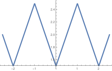 Fig.1: Graph of |x|
|
|
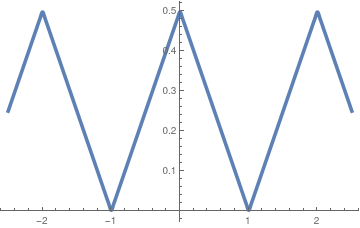 Fig.2: Graph of f(x)
|
|
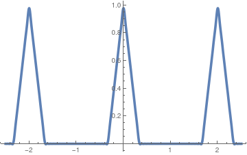 Fig.3: Graph of g(x)
|
s20[x_] =
2 - (4/Pi^2)*Sum[Cos[Pi*(2*k - 1) *x]/(2*k - 1)^2 , {k, 1, 20}];
Plot[s20[x], {x, -2.5, 2.5}, PlotStyle -> Thickness[0.01]]
s40[x_] =
1/4 + (2/Pi^2)*
Sum[ Sin[(n \[Pi])/2]^2 *Cos[Pi*n*x]/(n)^2 , {n, 1, 40}];
Plot[s40[x], {x, -2.5, 2.5}, PlotStyle -> Thickness[0.01]]
s30[x_] =
1/6 + (6/Pi^2)*
Sum[ (1 - Cos[n*Pi/3]) *Cos[Pi*n*x]/(n)^2 , {n, 1, 30}];
Plot[s30[x], {x, -2.5, 2.5}, PlotStyle -> Thickness[0.01]]
■
\begin{align*}
x &= - \frac{2\ell}{\pi} \sum_{n\ge 1} \frac{(-1)^n}{n}\,\sin \left( \frac{n\pi x}{\ell} \right) , \qquad 0 < x < \ell ,
\\
&= - \frac{4\ell}{\pi^2} \sum_{k\ge 1} \frac{1}{(2k-1)^2}\,\cos \left( \frac{\left( 2k-1 \right) \pi x}{\ell} \right) , \qquad 0 < x < \ell .
\end{align*}
2*Integrate[x*Sin[Pi*n*x/L], {x, 0, L}]/L
(2 L (-n \[Pi] Cos[n \[Pi]] + Sin[n \[Pi]]))/(n^2 \[Pi]^2)
\begin{align*}
x^2 &= \frac{2\ell^2}{\pi^3} \sum_{n\ge 1} \frac{-2 +(-1)^n \left( 2- n^2 \pi^2 \right)}{n^3}\,\sin \left( \frac{n\pi x}{\ell} \right) , \qquad 0 < x < \ell ,
\\
&= \frac{\ell^2}{3} + \frac{4\ell^2}{\pi^2} \sum_{n\ge 1} \frac{(-1)^n}{n^2}\,\cos \left( \frac{n\pi x}{\ell} \right) , \qquad 0 < x < \ell .
\end{align*}
2*Integrate[x^2 *Cos[n*Pi*x/L], {x, 0, L}]/L
(2 L^2 (2 n \[Pi] Cos[n \[Pi]] + (-2 + n^2 \[Pi]^2) Sin[
n \[Pi]]))/(n^3 \[Pi]^3)
Return to Mathematica page
Return to the main page (APMA0340)
Return to the Part 1 Matrix Algebra
Return to the Part 2 Linear Systems of Ordinary Differential Equations
Return to the Part 3 Non-linear Systems of Ordinary Differential Equations
Return to the Part 4 Numerical Methods
Return to the Part 5 Fourier Series
Return to the Part 6 Partial Differential Equations
Return to the Part 7 Special Functions