Return to computing page for the first course APMA0330
Return to computing page for the second course APMA0340
Return to Mathematica tutorial for the first course APMA0330
Return to Mathematica tutorial for the second course APMA0340
Return to the main page for the first course APMA0330
Return to the main page for the second course APMA0340
Return to Part III of the course APMA0340
Introduction to Linear Algebra with Mathematica
Glossary
Miscellany
Belousov–Zhabotinsky reaction
A Belousov–Zhabotinsky reaction, or BZ reaction, is one of a class of reactions that serve as a classical example of non-equilibrium thermodynamics, resulting in the establishment of a nonlinear chemical oscillator. The only common element in these oscillators is the inclusion of bromine and an acid. The reactions are important to theoretical chemistry in that they show that chemical reactions do not have to be dominated by equilibrium thermodynamic behavior. These reactions are far from equilibrium and remain so for a significant length of time and evolve chaotically
|
|
|
||
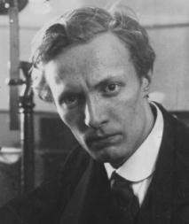
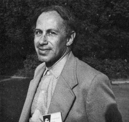
| Boris Pavlovich Belousov (1893--1970) | Belousov–Zhabotinsky reaction | Anatol Markovich Zhabotinsky (1938--2008) |
The Belousov-Zhabotinskii (BZ) reaction is an intriguing scillation that displays unexpected behavior. Full understanding of oscillatory behavior of chemical reactions is outside of the school curriculum. However, the importance of such processes in life sciences and peculiar spatial and temporal patterns accompanying the reactions can attract the attention of students. The famous Belousov–Zhabotinsky (BZ) dynamic system is \begin{align} \varepsilon\,\frac{{\text d}x}{{\text d}t} &= qy -xy + x \left( 1 - x \right) , \notag \\ \delta\,\frac{{\text d}y}{{\text d}t} &= -q\,y -xy +f\,z , \label{EqChaos.3} \\ \frac{{\text d}z}{{\text d}t} &= x-z . \notag \end{align}
- Barzykina, I., Chemistry and Mathematics of the Belousov–Zhabotinsky Reaction in a School Laboratory, Journal of Chemical Education, 2020, Vol. 97, No. 7, pp. 1895--1902. https://doi.org/10.1021/acs.jchemed.9b00906
- Belousov, B. P., Collection of short papers on radiation medicine for 1958; Medgiz: Moscow, 1959; pp. 145−147.
- Epstein, I. R. Obituary: Anatol Zhabotinsky (1938−2008).Nature, 2008,455, 1053.
- Field, R. J.; Körös, E.; Noyes, R. M., Oscillations in chemical systems. II. Thorough analysis of temporal oscillation in the bromate-cerium-malonic acid system., J. Am. Chem. Soc.1972, 94, pp. 8649−8664
- Field, R. J.; Noyes, R. M. Oscillations in Chemical Systems. IV.Limit Cycle Behavior in a Model of a Real Chemical Reaction., J. Chem.Phys.1974, 60, pp. 1877−1884.
- Györgyi, L.; Turánui, T.; Field, R. J. Mechanistic details of the oscillatory Belousov-Zhabotinskii reaction., J. Phys. Chem. 1990, 94, pp. 1931--1941.
- Tyson, J. J. Relaxation oscillations in the revised Oregonator, J.Chem. Phys.1984,80, 6079−6082.
- Zhabotinsky, A. M., Periodic oxidation of malonic acid in solution(a study of the Belousov reaction kinetics). Biofizika, 1964, 9, 306−311.
- Epstein, I.R., Pojman, J.A. An Introduction to Nonlinear Chemical Dynamics: Oscillations, Waves, Patterns, and Chaos. 1998. Oxford University Press. Oxford.
- Field, R.J., Noyes, R.M. Oscillations in chemical systems. IV. Limit cycle behavior in a model of a real chemical reaction. 1974. J. chem. Phys. 60, 1877-1884.
- Field, R.J. Oregonator. 2007. Scholarpedia 2(5).1386.
- Gyorgyi, L., Field, R.J. Simple Models of Deterministic Chaos in the Belousov-Zhabotinsky Reaction. 1991. J. chem Phys. 95, 6594-6602
- Gyorgyi, L., Field, R.J. A three-variable model of deterministic chaos in the Belousov-Zhabotinsky reaction. 1992. Nature 355, 808-810.
- Li, Y.N. Song, H. Cai, Z.S., Chen, L. Hou, Z., Wei, Q.L., Wu, B., Zhao, X.Z. New Chaotic Behavior and its effective control in Belousov-Zhabotinsky reaction. 2001. Can. J. Chem. 79, 29-34.
- Ren, J. Gao, J. Yang, Wu. Computational simulation of Belousov-Zhabotinskii oscillating chemical reaction. 2008. Computing And Visualization in Science 12, 227-234. Springer-Verlag.
- Scott, S.K. Chemical Chaos. 1991. Clarendon Press. Oxford.
- Swathi, B., Kulkarni, V.R. Simulation of a Few Bifurcation Phase Diagrams of Belousov-Zhabotinsky Reaction with Eleven Variable Chaotic Model in CSTR. 2009. E-Journal of Chemistry 6, 481-488.
The Martiel-Goldbeter system of ODEs is models the production of the signalling molecule cAMP by Dictyostelium discoideum. It has a remarkable life cycle, incorporating key features of morphogenesis in higher organisms. \begin{align*} \frac{{\text d} w_1}{{\text d}t} &= \alpha_4 u_2 - w_1 - \alpha_4 u_2 w_1 , \\ \frac{{\text d} w_2}{{\text d}t} &= \beta_2 \beta_3 c_2 u_4 - \beta_5 c_3 w_3 - c_3 \beta_4 u_1 u_2 - \beta_2 \beta_3 c_2 u_4 \left( w_2 + c_3 w_3 \right) , \\ \frac{{\text d} w_3}{{\text d}t} &= - \left( \beta_5 + \beta_6 \right) w_3 + \beta_4 u_1 w_2 , \\ \frac{{\text d} C_i}{{\text d}t} &= \gamma_1 \gamma_2 w_1 + \gamma_5 \left( 1 - w_1 \right) - \gamma_4 \frac{C_i}{C_i + \gamma_3} -sr(C_i ) , \\ \frac{{\text d} C_o}{{\text d}t} &= \Delta_1 \nabla^2 C_o - \gamma_9 \frac{C_o}{C_o + \gamma_8} + \frac{\rho}{1-\rho} \left( sr(C_i ) - \gamma_7 \frac{C_o}{C_o + \gamma_6} \right) , \end{align*} where \[ u_1 = \frac{\alpha_0 C_0 + \left( \beta_5 - \alpha_0 C_o \right) w_3}{\alpha_1 + \alpha_0 C_o + \beta_4 w_2} , \quad u_2 = \frac{\alpha_2 \alpha_5 c_1 u_1 \left( 1- w_1 \right)}{1+ \alpha_4 + \alpha_2 \alpha_3 c_1 u_1 - \alpha_4 w_1} , \quad u_4 = \frac{\beta_0 C_o}{\beta_1 + \beta_0 C_o} . \]
Shilnikov sense chaos
The Shilnikov homoclinic orbits appear in three dimesional (3D) systems of ODEs.
- Shilnikov, L.,P., A contribution to the problem of the structure of an extended neighbourhood of a rough state of saddle-focus type, Mathematics USSR Sbornik, 1970, Vol. 10, pp. 91--102.
- 1
- Wang, W., Zhang, Q.-C., and Tian, R.-L., Shilnikov sense chaos in a simple three-dimensional system, Chinese Physics B, March 2010, Vol. 19, No. 3, 030517; doi: 10.1088/1674-1056/19/3/030517
Return to Mathematica page
Return to the main page (APMA0340)
Return to the Part 1 Matrix Algebra
Return to the Part 2 Linear Systems of Ordinary Differential Equations
Return to the Part 3 Non-linear Systems of Ordinary Differential Equations
Return to the Part 4 Numerical Methods
Return to the Part 5 Fourier Series
Return to the Part 6 Partial Differential Equations
Return to the Part 7 Special Functions