Return to computing page for the first course APMA0330
Return to computing page for the second course APMA0340
Return to Mathematica tutorial for the first course APMA0330
Return to Mathematica tutorial for the second course APMA0340
Return to the main page for the first course APMA0330
Return to the main page for the second course APMA0340
Return to Part VII of the course APMA0340
Introduction to Linear Algebra with Mathematica

Preface


Legendre's polynomials are eigenfunctions of a singular Sturm--Liouville problem for a second order differential equation. They are named after Adrien-Marie Legendre, who discovered them in 1782. Adrien-Marie Legendre (1752--1833) was a French mathematician. Legendre made numerous contributions to mathematics. His major work is Exercices de Calcul Intégral, published in three volumes in 1811, 1817, and 1819, where he introduced the basic properties of elliptic integrals, beta functions and gamma functions, along with their applications to mechanics.

Legendre Equation


Adrien-Marie Legendre
The Legendre equation is the second order differential equation with a real parameter λ
\[ \left( 1-x^2\right) y'' -2x\,y' + \lambda\, y =0 , \qquad -1 < x < 1 . \]
This equation has two regular singular points x = ±1 where the leading coefficient (1 − x²) vanishes. Upon adding the boundary conditions and rewriting the equation in self-adjoint form, we obtain the Sturm--Liouville problem
\begin{equation} \label{EqLegendre.1} \frac{\text d}{{\text d}x} \left[ \left( 1- x^2 \right) \frac{{\text d} y}{{\text d}x} \right] + \lambda\, y =0 , \qquad y(-1) < \infty , \quad y(1) < \infty . \end{equation}
Eq.\eqref{EqLegendre.1} has two linear independent solutions, one of which must be unbounded at endpoints. It turns out that the Legendre equation has a bounded solution only when λ = n(n + 1) for some nonzero integer n ∈ ℤ+. Such value of parameter λ is called eigenvalue and corresponding (bounded) eigenfunction is known as the Legendre polynomial, denoted as Pn(x). Any bounded solution of the Legendre equation is a constant multiple of Pn(x).

Legendre Polynomials


A polynomial solution to the Legendre differential equation

\begin{equation} \label{EqLegendre.2} \left( 1-x^2\right) y'' -2x\,y' + n(n+1)\, y =0 \qquad\mbox{or} \qquad \frac{\text d}{{\text d}x} \left[ \left( 1- x^2 \right) \frac{{\text d} y}{{\text d}x} \right] + n(n+1)\, y =0 , \end{equation}
where n is a nonzero integer, was considered in section xvi of Part V in the first tutorial. It was shown that Eq.\eqref{EqLegendre.1} has a series solution
\[ y(x) = \sum_{k\ge 0} c_k x^k , \] with coefficients connected via the recurrence
\[ c_{k+2} = \frac{k \left( k+1 \right) - \lambda}{\left( k+1 \right)\left( k+2 \right)}\, c_k , \qquad k=0,1,2,\ldots . \] When λ = n(n + 1) for some nonzero integer n, Eq.\eqref{EqLegendre.1} has a polynomial solution, denoted by Pn(x) and called after Legendre. Each Legendre polynomial may be expressed using Rodrigues' formula (named after Benjamin Olinde Rodrigues (1795--1851), a French banker, mathematician, and social reformer):
\begin{equation} \label{EqLegendre.3} P_n (x) = \frac{1}{2^n n!} \,\frac{{\text d}^n}{{\text d}x^n} \left( x^2 -1 \right)^n , \qquad n=1,2,\ldots . \end{equation}

They also admit "explicit" expression:

\begin{equation} \label{EqLegendre.4} P_n (x) = \frac{1}{2^n} \sum_{k=0}^{\lfloor n/2 \rfloor} \frac{(-1)^k \left( 2n -2k \right)!}{k! \left( n-k \right)! \left( n -2k \right)!}\, x^{n-2k} , \qquad n=1,2,\ldots ; \end{equation}
where ⌊ · ⌋ is the floor function. The Legendre polynomials are built into Mathematica. Mathematica's notation is LegendreP[n,x] for Pn(x).

Example 1: We now use Mathematica to obtain the formulas for the first 11 of these polynomials. We put them in a table.

TableForm[Table[{i, i*(i + 1), LegendreP[i, x]}, {i, 0, 10}], TableHeadings -> {None, {"n", "\[Lambda]_k", "P_n (x)"}}]
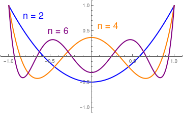
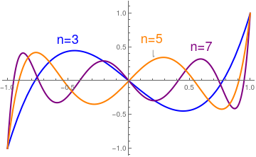
To get some idea of what these polynomials look like, we construct graphs of the first 7. We first define a function legraph[n] that produces a graph of the kth polynomial, and then we use a Do loop to construct the first 7 graphs.
legraph[n_] := Plot[LegendreP[n, x], {x, -1, 1}, AxesLabel -> {"x", "P_n (x)"}, PlotRange -> {{-1.1, 1.1}, {-1.1, 1.1}}, PlotLabel -> Row[{"n=", PaddedForm[n, 3]}]]
GraphicsGrid[Table[{legraph[i], legraph[i + 1]}, {i, 0, 6, 2}]]
First, we plot some Legendre polynomials using standard Mathematca input:
even = Plot[{LegendreP[2, x], LegendreP[4, x], LegendreP[6, x]}, {x, -1, 1}, PlotRange -> {{-1.1, 1.1}, {-1.1, 1.1}}, PlotStyle -> {{Thick, Blue}, {Thick, Orange}, {Thick, Purple}}];
t2 = Graphics[{Text[ Style["n = 2", FontSize -> 18, FontColor -> Blue], {-0.7, 0.8}]}];
t4 = Graphics[{Orange, Text[Style["n = 4", FontSize -> 18, FontColor -> Orange], {0.2, 0.6}]}];
t6 = Graphics[{Purple, Text[Style["n = 6", FontSize -> 18, FontColor -> Purple], {-0.4, 0.5}]}];
Show[even, t2, t4, t6]
and
Plot[{LegendreP[3, x], LegendreP[7, x], Callout[LegendreP[5, x], Style["n=5", 18, Orange], {.2, .35}]}, {x, -1, 1}, PlotStyle -> {{Blue, Thick}, {Purple, Thick}, {Orange, Thick}}, Epilog -> {{Text[Style["n=3", 18, Blue], {-0.5, 0.6}]}, {Text[ Style["n=7", 18, Purple], {0.6, 0.5}]}}]
     
Legendre's polynomials for n = 2, 4, 6.       Legendre's polynomials for n = 3, 5, 7.

First we set up a series to work with:

y = Sum[c[i] x^i, {i, 0, 6}] + O[x]^7
Out[1]= c[0] + c[1] x + c[2] x^2 + c[3] x^3 + c[4] x^4 + c[5] x^5 +
c[6] x^6 + O[x]^7

To see that our input is correct we type

OutputForm[y]//Normal

We are going to insert this series into the differential equation

de = (1 -x^2) D[y, {x,2}] - 2 x D[y,x] + 20 y == 0
Out[2]= (20 c[0] + 2 c[2]) + (18 c[1] + 6 c[3]) x + (14 c[2] + 12 c[4])
x^2 + (8 c[3] + 20 c[5]) x^3 + 30 c[6] x^4 + O[x]^5 == 0
Then we get the coefficients
coeffeqns = LogicalExpand[de]
Out[3]= 20 c[0] + 2 c[2] == 0 && 18 c[1] + 6 c[3] == 0 &&
14 c[2] + 12 c[4] == 0 && 8 c[3] + 20 c[5] == 0 && 30 c[6] == 0
and express through first two c[0] and c[1]:
solvedcoeffs = Solve[ coeffeqns, Table[ c[i], {i,2,12}]]

Solve::svars: Equations may not give solutions for all "solve" variables. >>

Out[4]= {{c[2] -> -10 c[0], c[3] -> -3 c[1], c[4] -> (35 c[0])/3, c[5] -> (6 c[1])/5, c[6] -> 0}}
Put these back into the series expansion.
y = y /. solvedcoeffs
Out[5]= { c[0] + c[1] x -10 c[0] x^2 - 3 c[1] x^3 + (35/3) c[0] x^4 + (6/5) c[1] x^5 + O[x]^7 }
Extract out the two linearly independent solutions
Coefficient[ y, c[0]]
Out[6]= {1 - 10 x^2 + (35 x^4)/3}
Coefficient[ y, c[1]]
Out[7]= {x - 3 x^3 + (6 x^5)/5}
To check our answer, we use Mathematica again because it knows Legendre:
LegendreP[4,x]
Out[8]= 1/8 (3 - 30 x^2 + 35 x^4)
This is different from the polynomial obtained earlier, but only by a constant factor. The constant factor is used to set the normailization for the Legendre polynomials.

End of Example 1
   ■
There are known many integral representations for Legendre's polynomials. we mention one of them, derived byLaplace:
\[ P_n (x) = \frac{1}{\pi} \int_0^{\pi} \left( x + \sqrt{1 - x^2} \,\cos\theta \right)^n {\text d}\theta , \qquad |x| \lt; 1. \]
There are some interesting values
\[ \int_0^1 P_n (x)\,{\text d}x = \begin{cases} 1 , & \ \mbox{ if}\quad n=0, \\ 0 , & \ \mbox{ if}\quad n= 2k, \quad k > 0, \\ (-1)^k \frac{(2k)!}{2^{2k+1} k! \left( k+1 \right)!} , & \ \mbox{ if}\quad n = 2k+1 ; \end{cases} \qquad \int_0^1 x\,P_n (x)\,{\text d}x = \begin{cases} 0 , & \ \mbox{ if}\quad n=2k+1 , \\ \frac{(-1)^k \left( 2k-2 \right)!}{4^k \left( k-1 \right)! \left( k+1 \right)!} , & \ \mbox{ if}\quad n= 2k. \end{cases} \qquad \]

We check validity of these two formulas with Mathematica
Integrate[LegendreP[5, x], {x, 0, 1}]
1/16
4!/2^5/2/6
1/16
Integrate[LegendreP[6, x], {x, 0, 1}]Integrate[LegendreP[6, x], {x, 0, 1}]
0
and
Integrate[x*LegendreP[6, x], {x, 0, 1}]Integrate[LegendreP[6, x], {x, 0, 1}]
1/128
4!/4^3/2/4!
1/128
Integrate[x*LegendreP[7, x], {x, 0, 1}]Integrate[LegendreP[6, x], {x, 0, 1}]
0

Formula \eqref{EqLegendre.4} shows that Legendre's polynomials contain only even or odd powers of x, depending on parity of n. From it, we derive the numerical values:

\[ P_n (1) = 1 , \qquad P_n (-1) = (-1)^n , \qquad P_{2n} (0) = (-1)^n \,\frac{(2n)!}{2^{2n} \, (n! )^2} ,\qquad P'_{n} (1) = \frac{n(n+1)}{2} , \qquad n=0,1,2,\ldots . \]

The leading coefficient (a multiple of xn in Pn(x)) of the Legendre polynomial or order n is

\[ P_n (x) = \frac{(2n)!}{2^n \left( n! \right)^2}\, x^n + \cdots . \]

The function

\[ u(\theta ) = u_n (\theta ) = \left( \sin\theta \right)^{1/2} P_n (\cos\theta ) , \qquad 0 \le \theta \le \pi ; \]
is a solution of the differential equation
\[ u'' + \frac{1}{4\,\sin^2 \theta}\,u + \left( n + \frac{1}{2} \right)^2 u = 0 , \qquad n = 0,1,2,\ldots . \]
We check it for n = 7:
u[t_] = Sqrt[Sin[t]]*LegendreP[7, Cos[t]];
Simplify[D[u[t], t, t] + u[t]/4/(Sin[t])^2 + (7 + 1/2)^2 *u[t]]
0

Example 2:

End of Example 2
   ■

Legendre Functions of Second Kind


Another linearly independent solution of Legendre's equation (see section ix in Part IV of tutorial I) when λ = n(n + 1) is conventionally denoted by Qn(x) and it can be determined from the formula (up to arbitrary constant multiple)

\begin{equation} \label{EqLegendre.5} Q_n (x) = P_n (x) \int \frac{{\text d}x}{P_n^2 (x)} \, \exp \left\{ \int \frac{2x}{1 - x^2}\,{\text d}x \right\} = P_n (x) \int \frac{{\text d}x}{P_n^2 (x) \left( 1 - x^2 \right)} = \frac{1}{2}\, P_n (x)\,\ln \frac{1+x}{1-x} + R_{n-1} (x) , \end{equation}
(* checking for n = 3 *)
LegendreP[3, x]*Integrate[1/(1 - x^2)/(LegendreP[3, x])^2, x]
LegendreQ[3, x]
Simplify[LegendreQ[3, x] - LegendreP[3, x]*Integrate[1/(1 - x^2 )/(LegendreP[3, x])^2, x]]
0
for some polynomial Rn-1(x) of degree n−1:
\begin{equation} \label{EqLegendre.6} R_{n-1} (x) = \sum_{k=1}^n \frac{1}{k}\,P_{k-1} (x)\,P_{n-k} (x) = \sum_{k=1}^{\lfloor (n+1)/2 \rfloor} \frac{2n-4k+3}{\left( 2k-1 \right) \left( n-k+1 \right)}\, P_{n-2k+1} (x) , \end{equation}
where ⌊ · ⌋ is the floor function. This function Qn(x) is called the Legendre function of the second kind. Mathematica has a build-in command for this function: LegendreQ[n, x].

Using Mathematica, we generate several Legendre polynomials of the second kind.

Sum[(1/k)*LegendreP[k - 1, x]*LegendreP[4 - k, x], {k, 1, 4}]
       n     Legendre function of the second kind
    n = 0         \( \displaystyle Q_0 (x) = \frac{1}{2} \, \ln\frac{x+1}{x-1} \)
    n = 1         \( \displaystyle Q_1 (x) = \frac{x}{2} \, \ln\frac{x+1}{x-1} -1 \)
    n = 2         \( \displaystyle Q_2 (x) = \frac{3\,x^2 -1}{4} \, \ln\frac{x+1}{x-1} - \frac{3}{2}\,x \)
    n = 3         \( \displaystyle Q_3 (x) = \frac{5\,x^3 - 3x}{4} \,\ln\frac{x+1}{x-1} - \frac{5}{2}\, x^2 + \frac{2}{3} \)
    n = 4         \( \displaystyle Q_4 (x) = \frac{35\,x^4 - 30\,x^2 +3}{16} \,\ln\frac{x+1}{x-1} - \frac{35}{8}\,x^3 + \frac{55}{24}\,x \)
    n = 5         \( \displaystyle Q_5 (x) = \frac{P_5 (x)}{2} \, \ln\frac{x+1}{x-1} - \frac{63}{8}\,x^4 + \frac{49}{8}\,x^2 - \frac{8}{15} \)
    n = 6         \( \displaystyle Q_6 (x) = \frac{P_6 (x)}{2} \, \ln\frac{x+1}{x-1} - \frac{231}{16}\,x^5 + \frac{119}{8}\,x^3 - \frac{231}{80}\,x \)
    n = 7         \( \displaystyle Q_7 (x) = \frac{P_7 (x)}{2} \, \ln\frac{x+1}{x-1} - \frac{429}{16}\,x^6 + \frac{275}{8}\,x^4 - \frac{849}{80}\,x^2 + \frac{16}{35} \)
    n = 8         \( \displaystyle Q_8 (x) = \frac{P_8 (x)}{2} \,\ln\frac{x+1}{x-1} - \frac{6435}{128}\,x^7 + \frac{9867}{128}\,x^5 - \frac{4213}{128}\,x^3 + \frac{15159}{4480}\,x \)
    n = 9         \( \displaystyle Q_9 (x) = \frac{P_9 (x)}{2} \,\ln\frac{x+1}{x-1} - \frac{12155}{128}\, x^8 + \frac{65065}{384}\, x^6 - \frac{11869}{128}\, x^4 + \frac{14179}{896}\, x^2 - \frac{128}{315} \)
    n = 10         \( \displaystyle Q_{10} (x) = \frac{P_{10} (x)}{2} \,\ln\frac{x+1}{x-1} - \frac{46189}{256}\, x^9 + \frac{70499}{192}\, x^7 - \frac{157157}{640}\, x^5 + \frac{26741}{448}\, x^3 - \frac{61567}{16128}\, x \)

We check with Mathematica

Q9[x_] = LegendreP[9, x]* Log[(x + 1)/(x - 1)]/2 - (128/315 - (14179 x^2)/896 + (11869 x^4)/ 128 - (65065 x^6)/384 + (12155 x^8)/128)
Simplify[(1 - x^2)*D[Q9[x], x, x] - 2*x*D[Q9[x], x] + 90*Q9[x]]
0

Associated Legendre Functons


The Legendre equation is a special case of the associated Legendre equation:
\begin{equation} \label{EqLegendre.7} \frac{\text d}{{\text d}x} \left[ \left( 1- x^2 \right) \frac{{\text d} y}{{\text d}x} \right] + \left( \lambda - \frac{m^2}{1-x^2} \right) y =0 , \qquad \lambda = n \left( n+1 \right) , \qquad x \in (-1, 1) . \end{equation}
Here m∈ℤ+ is a nonnegative integer. The Sturm--Liouville problem for Eq.\eqref{EqLegendre.7} asks to find such values of parameter λ for which solutions y(x) and its derivative \( \left( 1 - x^2 \right)^{1/2} y'(x) \) remain bounded at endpoints x = ±1. It turns out that this is possible only when λ = n(n+1), with n∈ℤ+. The eigenfunction corresponding to eigenvalues λn = n(n+1), n = 0, 1, 2, …, are convensionally called associated Legendre functions. They usually are denoted by \( P_n^m (x) , \quad m=0,1,2,\ldots , n; \) or by Pn(m, x). The function Pn(m, x) is a polynomial of degree n if and only if m is even. However, \( P_n^m (\cos\theta ) \) is a homogeneous polynomial of degree n in sinθ and cosθ. When m = 0, we get the Legendre equation.

The associated Legendre functions of the first kind are given by Rodrigue’s formula

\begin{equation} \label{EqLegendre.8} P_n^m (x) = \left( 1 - x^2 \right)^{m/2} \frac{{\text d}^m}{{\text d}x^m} \, P_n (x) = \left( 1 - x^2 \right)^{m/2} \frac{1}{2^n n!} \,\frac{{\text d}^{m+n}}{{\text d}x^{m+n}} \left( x^2 -1 \right)^n , \qquad m=0,1,2,\ldots , n . \end{equation}
Simplify[D[LegendreP[6, x], {x, 1}]]
21/8 x (5 - 30 x^2 + 33 x^4)

Mathematica has a build-in command to evaluate associated Legendre polynomials; however, it does not follow Eq.\eqref{EqLegendre.8}, but multiplies it by −1:

LegendreP[6, 1, 2, x]
-(21/8) Sqrt[1 - x] Sqrt[1 + x] (5 x - 30 x^3 + 33 x^5)
LegendreP[3, 3, 1, x]
-15 (1 - x^2)^(3/2)

Associated Legendre functions of second kind


Associated Legendre functions of the second kind are defined according to the formula
\begin{equation} \label{EqLegendre.9} Q_n^m (x) = \left( 1 - x^2 \right)^{m/2} \frac{{\text d}^m}{{\text d} x^m } \,Q_n (x) , \qquad n=m,m+1, m+2 , \ldots . \end{equation}

=====================================================================

Legendre functions


==================================================================

Example: solve the IVP:
(4-x^2 )y'[x]+y[x]==0, y[0]==1

Clear[a,n]
a[n_]:=a[n]=((n-2) a[n-2] -a[n-1])/4/n
a[0] = a0
a[1] = -a0/4
TableForm[Table[{n,a[n]},{n,0,5}]]
Out[21]/TableForm=
0 a0
1 -a0/4
2 a0/32
3 -3 a0/128
4 11 a0/2048
5 -31 a0/8192

When we apply the initial condition, we set a0=1 in the general solution.

Now we solve the initial value problem exactly:

Clear[x,y]
exactsol=DSolve[{(4-x^2)y'[x]+y[x]==0,y[0]==1},y[x],x]
Out[63]= {{y[x]-> (2-x)^(1/4)/(2+x)^(1/4) }}
Note that the exact solution is |2-x|^(1/4)/|2+x|^(1/4) with absolute values instead of parenthesis.

formula=Simplify[(2-x)^(1/4)/(2+x)^(1/4)]

Out[64]= (2 - x)^(1/4)/(2 + x)^(1/4)
var=Table[D[y[x],i]/.x->0,{i,1,11}]
????sols=Solve[sysofeqs,vars]
sersol=Series[y[x],{x,0,11}/.sols[[1]]]

Legendre's equation

genform =
Solve[(n + 2)*(n + 1)*a[n + 2] + (-n*(n - 1) - 2 n + k*(k + 1))*
a[n] == 0, a[n + 2]]
Out[8]= {{a[2 + n] -> -(((k + k^2 - n - n^2) a[n])/((1 + n) (2 + n)))}}
Factor[genform[[1, 1, 2]]]
Out[9]= ((-k + n) (1 + k + n) a[n])/((1 + n) (2 + n))
We obtain a formula for a[n] by replacing each occurrence of n in a[n+2] by n-2.
genform[[1, 1, 2]] /. n -> n - 2
Out[10]= -(((2 + k + k^2 - (-2 + n)^2 - n) a[-2 + n])/((-1 + n) n))
a[n_] := -(((2 + k + k^2 - (-2 + n)^2 - n) a[-2 + n])/((-1 + n) n))
DSolve[(1 - x^2)*y''[x] - 2 x y'[x] + k*(k + 1)*y[x] == 0, y[x], x]
Out[12]= {{y[x] -> C[1] LegendreP[k, x] + C[2] LegendreQ[k, x]}}


  1. Grigoryan, V, Partial Differential Equations, 2010, University of California, Santa Barbara.


Return to Mathematica page
Return to the main page (APMA0340)
Return to the Part 1 Matrix Algebra
Return to the Part 2 Linear Systems of Ordinary Differential Equations
Return to the Part 3 Non-linear Systems of Ordinary Differential Equations
Return to the Part 4 Numerical Methods
Return to the Part 5 Fourier Series
Return to the Part 6 Partial Differential Equations
Return to the Part 7 Special Functions