Preface
This chapter is about applications of numerical methods for solving systems of ordinary differential equations.
Return to computing page for the first course APMA0330
Return to computing page for the second course APMA0340
Return to Mathematica tutorial for the first course APMA0330
Return to Mathematica tutorial for the second course APMA0340
Return to the main page for the first course APMA0330
Return to the main page for the second course APMA0340
Introduction to Linear Algebra with Mathematica
Glossary
All engineering and practical achievements are based on the laws of physics that are exact expressions of an inexact universe. The laws of physics are translations of concrete observations into the ideal language of mathematics. This kinship between the concrete and the ideal is the highest intellectual achievement of mankind and the driving force behind our ability to unravel the secrets of the universe. However, in real life, we deal with objects that are not ideal. When humans want to make predictions based on appropriate models, they need to approximate the objects of the universe in such a way that the laws of physics could be applied to them. There are several known approaches for such approximations, and differential equations are currently the most successful tool in modelling.This part of the tutorial deals with nonlinear ordinary differential equations that are used to model in many practical problems. Differential equations are used to map all sorts of physical phenomena, from chemical reactions, disease progression, motions of objects, electronic circuits, weather forecast, et cetera. Most mathematical models of real-world situations do not have analytical solutions. It is well-known that only few ordinary differential equations have explicit solutions expressible in finite terms. This is not simply because ingenuity fails, but because the repertory of standard functions (polynomials, exponential, trigonometric and their inverses) in terms of which solutions may be expressed is too limited to accommodate the variety of differential equations encountered in practice. Even if a solution can be found, the ‘formula’ is often too complicated to display clearly the principal features of the solution; this is particularly true of implicit solutions and of solutions which are in the form of integrals or infinite series.
Numerical Methods
General numerical methods
Euler's algorithms
Polynomial approximations
Runge-Kutta methods
Multistep methods
Numerical methods for boundary value problems
a. Shooting method
b. Weighted residual method
c. Finite difference method
The abundant literature on the subject of numerical solution of ordinary differential equations is on the one hand, a result of the tremendous variety of actual systems in the physical and biological sciences and engineering disciplines that are described by ordinary differential equations and, on the other hand, a result of the fact that the subject is currently active. The existence of a large number of methods, each having special advantages, has been a source of confusion as to what methods are best for certain classes of problems. In many cases, it is possible to use a black box differential equations solver. However, in some cases, a black box method is inadequate.
One of the advantages of a numerical approach is that it is mathematically less difficult and therefore accessible to students at an earlier point in their studies. Numerical methods are also more powerful in that they permit the treatment of problems for which analytical solutions do not exist. A third advanatage is that the numerical approach may afford the student an insight into the dynamics of a system that would not be attained through the traditional analytical method of solution. However, there exist a tremendous number of discrete analogs corresponding to one continuous model, and many of them may exhibit properties that do not belong to its continuous counterpart.
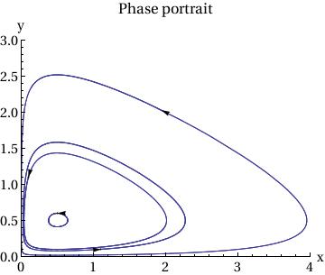
ParametricPlot[
Table[{x[t], y[t]} /. sol[[j]], {j, Length[ic]}], {t, 0, T},
PlotRange -> {{0, 4}, {0, 3}}],
Table[Graphics[{Arrowheads[.03],
Arrow[{ic[[j]], ic[[j]] + .01 f[ic[[j, 1]], ic[[j, 2]] ] }]}],
{j, Length[ic]}],
AxesLabel -> {"x", "y"},
BaseStyle -> {FontFamily -> "Times", FontSize -> 14},
PlotLabel -> "Phase portrait"
]
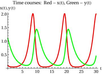
PlotStyle -> {{Thickness[0.01], RGBColor[1, 0, 0]}, {Thickness[0.01],
RGBColor[0, 1, 0]}}, AxesOrigin -> {0, 0},
AxesLabel -> {"t", "x(t),y(t)"},
BaseStyle -> {FontFamily -> "Times", FontSize -> 14},
PlotLabel -> "Time courses: Red - x(t), Green - y(t)"]
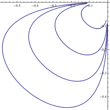
Example. Consider the system of autonomous equations
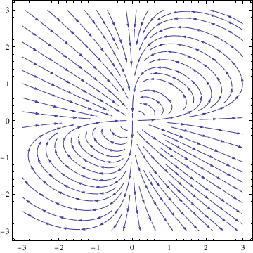
deq2 = y'[t] == 2*x[t]*y[t] - y[t]^2;
soln = NDSolve[{deq1, deq2, x[0] == 1, y[0] == 1}, {x[t], y[t]}, {t, -10, 10}];
Do[Clear[x, y];
soln = NDSolve[{deq1, deq2, x[0] == n/10, y[0] == n/10}, {x[t], y[t]}, {t, -10, 10}];
x = soln[[1, 1, 2]];
y = soln[[1, 2, 2]];
curve[[n]] = ParametricPlot[{x, y}, {t, -10, 10}, PlotStyle -> Thick], {n, -4, 4}];
Show[curve[[-4]], curve[[-3]], curve[[-2]], curve[[-1]], curve[[1]], curve[[2]], curve[[3]], curve[[4]], AspectRatio -> 1]
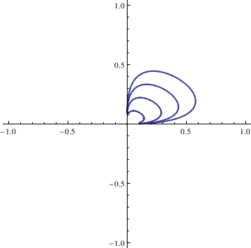
soln = NDSolve[{deq1, deq2, x[0] == n/10, y[0] == n/10}, {x[t], y[t]}, {t, -10, 10}];
x = soln[[1, 1, 2]];
y = soln[[1, 2, 2]];
curvep[[n]] = ParametricPlot[{x, y}, {t, -10, 10}, PlotStyle -> Thick], {n, 0, 4}];
Show[curvep[[0]], curvep[[1]], curvep[[2]], curvep[[3]], curvep[[4]], AspectRatio -> 1]
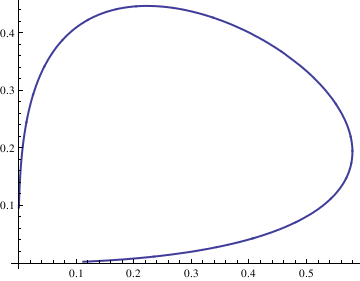
G[x_, y_] := x^3;
sol = NDSolve[{x'[t] == F[x[t], y[t]], y'[t] == G[x[t], y[t]],
x[0] == 1, y[0] == 0}, {x, y}, {t, 0, 3*Pi},
WorkingPrecision -> 20]
ParametricPlot[Evaluate[{x[t], y[t]}] /. sol, {t, 0, 3*Pi}]
Y[t_] := Evaluate[y[t] /. sol]
fns[t_] := {X[t], Y[t]};
len := Length[fns[t]];
Plot[Evaluate[fns[t]], {t, 0, 3*Pi}]
2.4.1. General Numerical Methods
G[x_, y_] := x^3;
sol = NDSolve[{x'[t] == F[x[t], y[t]], y'[t] == G[x[t], y[t]],
x[0] == 1, y[0] == 0}, {x, y}, {t, 0, 3*Pi},
WorkingPrecision -> 20]
ParametricPlot[Evaluate[{x[t], y[t]}] /. sol, {t, 0, 3*Pi}]
Y[t_] := Evaluate[y[t] /. sol]
fns[t_] := {X[t], Y[t]};
len := Length[fns[t]];
Plot[Evaluate[fns[t]], {t, 0, 3*Pi}]
- Lepik, Ü., Haar wavelet method for solving stiff differential equations, Mathematical Modelling and Analysis, 2009, Volume 14, Number 4, 2009, pages 467–481 ISSN 1648-3510; doi:10.3846/1392-6292.2009.14.467-481
Return to Mathematica page
Return to the main page (APMA0340)
Return to the Part 1 Matrix Algebra
Return to the Part 2 Linear Systems of Ordinary Differential Equations
Return to the Part 3 Non-linear Systems of Ordinary Differential Equations
Return to the Part 4 Numerical Methods
Return to the Part 5 Fourier Series
Return to the Part 6 Partial Differential Equations
Return to the Part 7 Special Functions